Mapping Particles to and from the Mesh
The previous section covered the short-ranged, "direct space" computation.
This section is the first of two that will cover the reciprocal space sum. For
the present discussion, we will treat the operations on the mesh, starting with
the forward three-dimensional Fast Fourier Transform (3DFFT) and ending with
the reverse 3DFFT, as a black box. The following page
will discuss the FFT operations and convolution.
The method of choice for mapping particles to and from the mesh is the
B-spline. These things have some notable properties: first, they are a
smooth partition of unity: the weights of all n knots in an
nth order spline add up to 1. The simplest B-spline
is a top hat function, the next simplest is a tent (pointy hat) function, and
very high order splines approximate a Gaussian / normal distribution. The
minimum smoothly differentiable spline has order 3, just above the tent
function, but these would require a very fine mesh or wide charge spreading
to offer precision in the final result, so the first (and sometimes only)
choice in Amber simulations is order 4, a cubic B-spline.
This order of the B-spline interpolation is indeed a critical
setting. Higher orders are available in the CPU versions of
sander and pmemd, but other than 4 the only other
truly useful order is 6. Each particle's position is interpolated using
B-splines in three dimensions, constructing a stencil of
n3 points, all weighted as the product of the three
splines' weights, implying that simulation costs scale as the cube of the
interpolation order. Raising the interpolation order, as stated in the
previous discussion, reduces the charge spreading factor to mesh spacing ratio,
allowing considerable savings in mesh density while keeping the short-ranged
cutoff small. More than 6, however, and the added cost is too much to justify.
Less than 4 and the savings in mapping costs are too small to justify the
accommodations that would be needed either in mesh density or the reach of the
short-ranged potential. Please inform your server if you would like four, or
six, and he will suggest solvent model pairings to suit your palette.
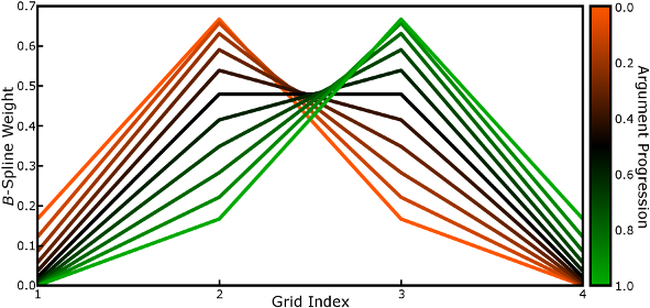
Each of the n B-spline coefficients has a unique value
determined by the argument, that is the alignment of the particle to the mesh
along each dimension. The argument is zero when a particle sits precisely on
a mesh point, grows towards 1 as the particle moves towards the next mesh
point, and then resets to zero as the stencil shifts by 1 mesh point. A
progression of the B-spline coefficients is shown below as the grid
alignment of a particle changes (the brightest orange line indicates the
weights when the particle is 0.0001 grid spacings past a mesh point, the
brightest green when it is 0.9999 towards the next mesh point). Code to
generate these spline weights is
here.
At least up to order 6, which again seems to be the highest order that is
useful in simulations, it is most efficient to compute B-splines and
their derivatives using a recurrence relation, as can be seen in the low-level
functions bspln and bsplnV (the second is merely a
vectorized form of the first, better suited for Matlab and Octave). The
derivatives of nth order B-splines, best calculated at
the (n-1)th application of the recurrence relation, are
readily found from the analytic forms and will later serve to calculate
gradients of the long-ranged, mesh-based potential.
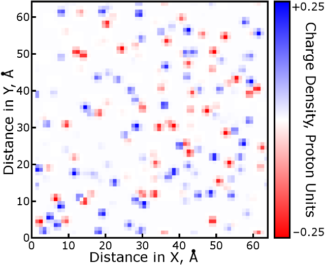
After computing B-spline coefficients in each direction for all
particles, it is time to multiply out the three-dimensional stencils and add
each particle's density to the mesh. Because B-splines are a
smooth partition of unity, the sum of the stencil points will equal 1 and can
then be scaled by the particle's partial charge. A slice of the charge
density mesh for the cubeions system in the Tests/
folder is displayed below. Real molecular simulations will have several
times the particle density and thus a more rugged density grid than this
example. Code to generate this figure can be found
here. Notice that it
closely follows the workflow of pmeRecip.m.
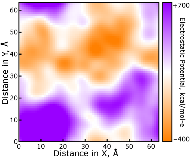
Once complete, the charge density mesh is convoluted with the potential
function dictating how one mesh point interacts with another. This convoultion
will be discussed in detail in the following section.
Here, we will simply make that happen with the pmeOrthoConvBC
function. The result is shown below, in terms of the electrostatic potential
that a test charge of one proton unit would experience. Due to the nature of
this example, randomly distributed ions of ∓1 proton charge, the field is
also somewhat stronger than will be seen in a typical simulation.
What happens in the convolution is the most mathematically demanding part
of Particle-Mesh Ewald, but understanding how to get particle information to
and from the mesh should make the general concept much less mysterious.
Go to the next section
Go to the previous section
|


