(Note: These tutorials are meant to provide
illustrative examples of how to use the AMBER software suite to carry out
simulations that can be run on a simple workstation in a reasonable period of
time. They do not necessarily provide the optimal choice of parameters or
methods for the particular application area.)
Copyright Ross Walker 2008
TUTORIAL A1
Simulating a Solvated Protein that Contains Non-Standard
Residues
(More Advanced Version)
By Ross Walker
In tutorials 1 to 3 all the systems we studied contained only standard amino acid or nucleic acid residues. As such we did not need to create units for non-standard residues and provide our own parameters. In this tutorial we will look at one method for creating a non-standard residue.
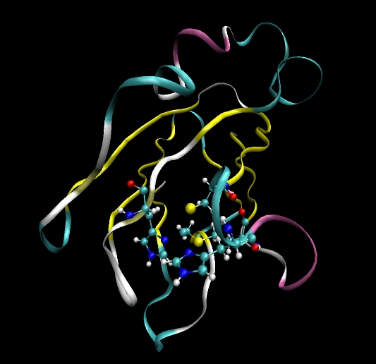
In this tutorial we will be aiming to setup a protein simulation of Plastocyanin in explicit solvent. In order to do this there are a number of things we will need to do:
Plastocyanin contains a copper ion (Cu) bound to four amino acids. His37, Cys84, His87 and Met92. We will need to modify these residues such that we can bind them to the copper ion. We will also need to supply parameters for these new bond types (and the corresponding angle and dihedral types these bonds create).
The PDB file for plastocyanin (1PLC) contains crystallographic waters which we should keep. However, only the oxygen positions are specified so we will use XLeap to add the missing protons. We will have to minimise these positions, however, before running production simulations.
Somewhat unusually the PDB file contains explicit protons for the protein. This is the same situation as tutorials 2 and 3, the proton naming convention used does not match IUPAC specifications. We need to correct this.
Using the most probable protonation states (at neutral pH) results in the Plastocyanin protein having an overal charge of -8. As such we will add 8 Na+ counterions around the system to neutralise it.
This will take a bit of work but it is significantly easier to do in AMBER 8 than it used to be.
Stage 1 - Do some editing of the PDB file.
The pdb file we will use is PDB ID: 1PLC - 1PLC.pdb.
You should always read all of the header information in a pdb file since it often contains important information about disordered pairs etc. Often 1 pdb file can also contain a series of different structures / inhibitors etc for the same protein system. In this pdb we see that waters #187 and #183 form a disordered pair and so both should not be present.
REMARK 4 1PLC 83 REMARK 4 HOH 187 AND HOH 183 FORM A DISORDERED PAIR AND BOTH ARE NOT 1PLC 84 REMARK 4 PRESENT SIMULTANEOUSLY. 1PLC 85 |
Thus I will arbitrarily remove water 187 from the pdb file and keep 183. I will also remove all of the connectivity data at the end of the PDB as this will not be used by XLeap. Each of our water molecules here is an individual resiude. Normally we need to add TER cards between residues that are not bound together in a chain. Fortunately we don't need to do that for our crystallographic waters since XLeap is smart enough to know that each of our waters is a separate molecule. This is defined in the WAT unit.
Since pdb files do not distinguish between cysteine residues that are involved in bonds or other things (and hence which have no proton on the sulphur atom) we need to edit the relevant cysteine residues to correct for this. The residue name used by Leap for regular protonated cysteine residues is CYS, for deprotonated (-ve charge) it is CYM and for cysteine residues involved in disulphide bridges and other bonds it is CYX. Since cysteine 84 in plastcyanin is bonded to the copper ion we need to change the residue name of residue 84 from CYS to CYX. The same is true for histidine residues which can be protonated in the 'delta' position (HID), the epsilon position (HIE) or at both (HIP). Fortunately in plastocyanin this is fairly easy since there are only two histidine residues (37 and 87) both of which are bonded to the copper via the 'delta' nitrogen. Thus they must both be protonated on the epsilon nitrogen. We are making our own unit (HIC) for residue 37 but we initially want it protonated on the epsilon nitrogen so we change it from HIS to HIE here. We also need to change the other histidine residue 87 from HIS to HIE.
Here is the modified pdb file so far: 1PLC_mod.pdb
The next stage before we can use the PDB is to sort out the non-standard hydrogen names. One option would be to simply strip out the protons and have XLeap add them back in at standard position as we did in the previous two tutorials. In this example though we shall try to keep the positions specified in the PDB file. We can use an AMBER tool for this called protonate. Protonate is typically used to protonate pdb files that do not have protons present. It can also be used, however, to correct pdb files that don't conform to IUPAC proton naming conventions. We run it as follows:
$AMBERHOME/exe/protonate -k -d $AMBERHOME/dat/PROTON_INFO -i 1PLC_mod.pdb -o 1PLC_mod2.pdb -l protonate.out
The -k option changes the names but "keeps" the positions as specified in the pdb file. The -d option specified the PROTON_INFO file that is in the dat directory of the AMBER 8 installation. This specifies information on where to place the protons. Protonate also strips all of the unnecessary header info for us.
The line above should produce the following files: 1PLC_mod2.pdb, protonate.out.
We don't need the protonate.out file but it is a good idea to take a look at it to check for any errors. In my case it was empty and so there were no errors or mysterious protons.
The next stage is to work out how we are going to treat the copper atom. In this example we shall make the copper atom part of residue 37. Residue HIE 37 will then become a non-standard residue, since it is now a histidine atom with a copper atom attached. Hence we will edit the pdb and move the copper atom from the end of the protein and place it as the last atom of residue 37. We also need to change its residue name to HIC and its residue number to 37. We also need to change all of the other atoms in residue 37 from HIE to HIC.
ATOM 527 N HIC 37 4.103 34.339 15.185 ATOM 528 H HIC 37 3.437 33.878 14.758 ATOM 529 CA HIC 37 4.992 33.545 15.990 ATOM 530 HA HIC 37 5.838 33.996 16.025 ATOM 531 C HIC 37 5.176 32.169 15.301 ATOM 532 O HIC 37 4.427 31.772 14.434 ATOM 533 CB HIC 37 4.395 33.294 17.344 ATOM 534 3HB HIC 37 4.944 32.577 17.764 ATOM 535 2HB HIC 37 3.447 32.920 17.176 ATOM 536 CG HIC 37 4.163 34.407 18.291 ATOM 537 ND1 HIC 37 5.162 35.218 18.775 ATOM 538 CD2 HIC 37 2.952 34.795 18.848 ATOM 539 HD2 HIC 37 2.063 34.452 18.734 ATOM 540 CE1 HIC 37 4.572 36.081 19.598 ATOM 541 HE1 HIC 37 5.044 36.764 20.072 ATOM 542 NE2 HIC 37 3.236 35.857 19.674 ATOM 543 HE2 HIC 37 2.630 36.345 20.187 ATOM 1444 CU HIC 37 7.050 34.960 18.716 |
For the methionine that is bound to the copper via a long bond (MET 92) we will create a new residue called MEM (a made up residue name that is not currently in use) that will have a sulphur of type SM rather than S. SM, is a type I just made up that we will use to create special force field parameters for MET 92's S-Cu bond. Thus we need to edit the pdb and change all of residue names for residue 92 from MET to MEM.
The original pdb file also contained several "alternate" configurations for some residues. E.g. for LYS 30 we had
ATOM 426 N LYS 30 -0.930 27.774 20.957 1.00 8.07 1PLC 549 ATOM 427 CA LYS 30 -2.028 28.602 20.421 1.00 10.86 1PLC 550 ATOM 428 C LYS 30 -1.629 30.029 20.254 1.00 9.16 1PLC 551 ATOM 429 O LYS 30 -1.226 30.665 21.243 1.00 7.63 1PLC 552 ATOM 430 CB ALYS 30 -3.201 28.489 21.415 0.50 13.41 1PLC 553 ATOM 431 CB BLYS 30 -3.250 28.517 21.354 0.50 15.09 1PLC 554 ATOM 432 CG ALYS 30 -4.397 29.366 21.249 0.50 16.84 1PLC 555 ATOM 433 CG BLYS 30 -4.600 28.495 20.646 0.50 21.50 1PLC 556 ATOM 434 CD ALYS 30 -5.681 28.891 21.893 0.50 20.64 1PLC 557 ATOM 435 CD BLYS 30 -5.745 28.171 21.589 0.50 24.43 1PLC 558 ATOM 436 CE ALYS 30 -5.527 28.212 23.225 0.50 23.18 1PLC 559 ATOM 437 CE BLYS 30 -5.585 26.973 22.460 0.50 24.88 1PLC 560 ATOM 438 NZ ALYS 30 -6.825 28.052 23.929 0.50 20.02 1PLC 561 ATOM 439 NZ BLYS 30 -5.971 25.681 21.860 0.50 26.52 1PLC 562 ATOM 440 H LYS 30 -0.661 27.945 21.802 1.00 8.96 1PLC 563 ATOM 441 HA LYS 30 -2.302 28.229 19.582 1.00 10.61 1PLC 564 ATOM 442 1HB ALYS 30 -3.380 27.572 21.665 0.50 14.09 1PLC 565 ATOM 443 1HB BLYS 30 -3.134 27.712 21.919 0.50 15.93 1PLC 566 ATOM 444 2HB ALYS 30 -2.700 28.880 22.297 0.50 13.96 1PLC 567 ATOM 445 2HB BLYS 30 -3.188 29.326 21.939 0.50 15.16 1PLC 568 ATOM 446 1HG ALYS 30 -4.210 30.316 21.598 0.50 18.44 1PLC 569 ATOM 447 1HG BLYS 30 -4.784 29.428 20.234 0.50 20.74 1PLC 570 ATOM 448 2HG ALYS 30 -4.609 29.538 20.265 0.50 17.98 1PLC 571 ATOM 449 2HG BLYS 30 -4.629 27.910 19.855 0.50 20.04 1PLC 572 ATOM 450 1HD ALYS 30 -6.278 29.712 22.058 0.50 21.47 1PLC 573 ATOM 451 1HD BLYS 30 -5.929 28.976 22.170 0.50 24.46 1PLC 574 ATOM 452 2HD ALYS 30 -6.224 28.346 21.263 0.50 21.94 1PLC 575 ATOM 453 2HD BLYS 30 -6.606 28.094 21.037 0.50 24.54 1PLC 576 ATOM 454 1HE ALYS 30 -5.138 27.298 23.130 0.50 22.69 1PLC 577 ATOM 455 1HE BLYS 30 -4.709 26.867 22.883 0.50 25.84 1PLC 578 ATOM 456 2HE ALYS 30 -4.956 28.735 23.845 0.50 23.28 1PLC 579 ATOM 457 2HE BLYS 30 -6.257 27.063 23.262 0.50 25.75 1PLC 580 ATOM 458 1HZ ALYS 30 -7.360 28.765 23.779 0.50 21.25 1PLC 581 ATOM 459 1HZ BLYS 30 -6.721 25.740 21.353 0.50 26.03 1PLC 582 ATOM 460 2HZ ALYS 30 -7.206 27.240 23.677 0.50 21.83 1PLC 583 ATOM 461 2HZ BLYS 30 -5.279 25.211 21.533 0.50 25.17 1PLC 584 ATOM 462 3HZ ALYS 30 -6.682 27.986 24.852 0.50 21.60 1PLC 585 ATOM 463 3HZ BLYS 30 -6.289 25.095 22.599 0.50 25.92 1PLC 586 |
By default Leap and protonate will use the A conformation and disregard the others. This is fine for our purposes here. If we specifically wanted to start out in one of the other confirmations we would need to remove the A conformation from the file.
The final thing we need to do is add a TER card between our last protein atom and our first crystallographic water atom.
Here is the pdb file after the modifications above: 1PLC_mod_final.pdb
Stage 2 - Creating the non-standard HIC and MEM units.
If simply loaded our edited pdb file above into XLeap at this point the vast majority of the file would load ok. There would be problems, however, with our two non-standard residues HIC and MEM. Before we can successfully load our 1PLC_modified_final.pdb file into XLeap we need to tell it what our two non-standard units are.
We have several options on how to deal with this. The easiest option for a simple molecule would be to use Antechamber as you will do in tutorial 5. Antechamber provides an automated method for creating non-standard units. However, it only works with complete molecules, not fragments as we have here.
A second option would be to simply edit the residues within xleap this once and then disregard them when we quit. This is the quickest method but doesn't allow for any re-use of our residues. E.g if we wanted to create a second very similar protein we would have to go through and repeat the process of editing the residues in xleap all over again.
The third option, and the one we will use here, is to create new library files for each of our non-standard units. In this way we can re-use those units, by simply loading the library files into xleap before we load our protein pdb, for similar proteins.
So, if you haven't already, fire up xleap and load our 1PLC_mod_final.pdb file into a new unit called PLC.
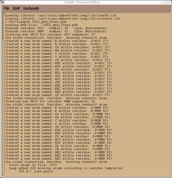
$AMBERHOME/exe/xleap -s -f $AMBERHOME/dat/leap/cmd/leaprc.ff99
> 1PLC=loadpdb 1PLC_mod_final.pdb
We should check the messages xleap gives us to ensure it has done what we expected. It should report only two unknown residues, our HIC and MEM. It should also have added any missing protons. Since we already ran our pdb through protonate the only missing atoms should be the protons on the our 109 water molecules. Hence we expect xleap to add a total of 218 H atoms. Verify that this is indeed the case. If it isn't then you missed something during the pdb edit. There should also have been 35 atoms that were not in residue templates, these are 18 in our HIC residue and 17 in our MEM residue. This is just a test to check everything is okay. We can quit xleap now.
Creating MEM and HIC units
We now need to create library files for our MEM and HIC units. The quickest way to do this, since we need initial structures for these units, is to simply cut them out of the 1PLC_mod_final.pdb file and save them as their own pdb files.
Now we can go ahead and load xleap again (are you getting good at this yet? :-)) and load the two pdb files into their own units:
$AMBERHOME/exe/xleap -s -f $AMBERHOME/dat/leap/cmd/leaprc.ff99
> HIC = loadpdb hic.pdb
> MEM = loadpdb mem.pdb
Now we need to tell xleap about our non-standard residues. We need to tell it what is bonded to what, what the atom types are and what the point charges on the atoms are. Lets start with the modified methionine residue.
> edit MEM
This should bring up our MEM residue in the editing window, you can turn on atom names with the Display menu.
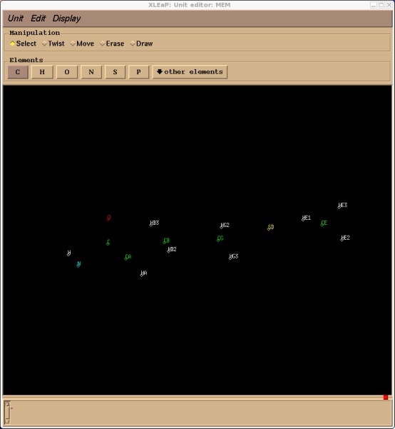
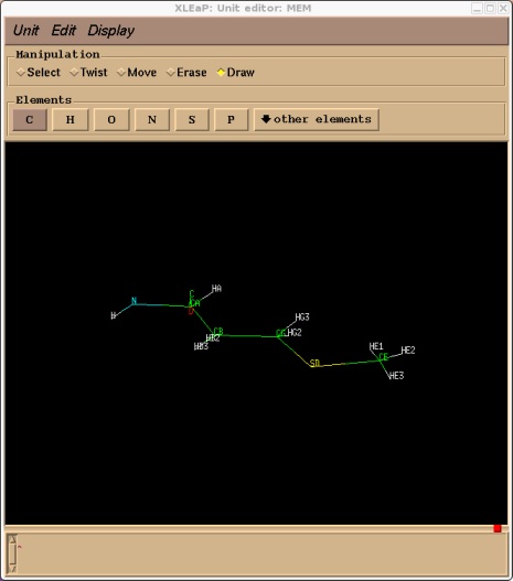
As you can see xleap currently knows nothing about the bonding within this residue. We can correct that quickly by simply drawing in the bonds. On the manipulation bar near the top of the edit window select draw and then connect the atoms as they should be bonded within methionine (remember, hold middle button to rotate, and middle + right to zoom in and out).
H->N->CA->C->O
CA->HA
CA->CB->HB3
CB->HB2
CB->CG->SD
CG->HG2
CG->HG3
SD->CE->HE1
CE->HE2
CE->HE3
Note, once you are proficient with AMBER you can copy prep files from the default units and modify these and therefore save yourself a lot of time. For the purposes of this tutorial it easier to understand what is going on if we do it from scratch. Here is the finished product:
At this point we should save a library file of what we have done so far. In this way if we make a mistake we can simply quit, load xleap again, load the library file and carry on from where we were. Go back to the command window and type:
saveoff MEM mem.lib
Now go back to the edit window. The next step is to specify the atom types and charges.
Typically you would need to calculate atomic charges for the copper atom and all of the other atoms in our HIC residue and also the MEM residue. This is necessary because the presence of the copper atom will alter the electron distribution in these surrounding residues. For AMBER this is done using the Restrained Electrostatic Potential Method (RESP). Details of calculating RESP charges can be found on the AMBER website. I will not cover this step in this tutorial, you will just have to trust me on the charge assignments. Note, the RESP fitting procedure has now been automated with a free program called R.E.D. Details of how to obtain and use R.E.D are available at http://www.u-picardie.fr/labo/lbpd/RED/.
For the purposes of this tutorial we will use the charges shown in the screen shot below. In order to specify the charges and atom types we need to select the entire unit. Hit the select button in the Manipulation bar and then rubberband the entire molecule. It should all change colour. Then go to the Edit menu:
Edit->Edit Selected Atoms
The following box should come up.
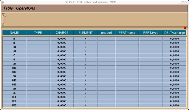
You should now go through and assign an atom type and charge for all of the atoms. For the charges you can use the ones shown below that I have calculated for you. For the atom types I have simply used all of the same atom types as defined in a regular MET unit (try editing MET if you want to see them) with the exception of the sulphur atom SD which, as mentioned earlier, I have made type SM. So edit the table so it looks like this (or if you don't have time just read on and I will give you the library file at the end).
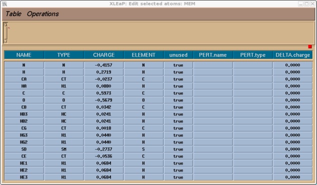
Once this is done we can select Table->Save and Quit. We can then close the edit window we should just be left with the command window. The last thing we need to do before we can save a library file for our completed unit is to tell xleap what is the head atom for this unit and what is the tail atom. This information is used in order to connect the protein back bone. E.g. if we type desc MEM we will see that there is no head or tail defined:
> desc MEM
UNIT name:
Head atom: null
Tail atom: null
.
.
.
However, if we look at MET we shall see that the backbone N is defined as the Head and the backbone C is defined as the Tail:
> desc MET
UNIT name: MET
Head atom: .R<MET 1>.A<N 1>
Tail atom: .R<MET 1>.A<C 16>
.
.
.
So we need to specify these for our MEM unit. Type:
> set MEM head MEM.MEM.N
> set MEM tail MEM.MEM.C
And that's us done. Now we can save the completed library file:
> saveoff MEM mem.lib
Here it is: mem.lib
We should now repeat the entire process for our HIC residue. To save you time though I have done it for you already. In creating the bonds I ensured that I bound the copper atom CU to the delta nitrogen ND1. The atoms types and charges I assigned were:
| ATOM | TYPE | CHARGE |
| N | N | -0.3479 |
| H | H | 0.2747 |
| CA | CT | -0.1354 |
| HA | H1 | 0.1212 |
| C | C | 0.7341 |
| O | O | -0.5894 |
| CB | CT | -0.0414 |
| HB3 | HC | 0.0810 |
| HB2 | HC | 0.0810 |
| CG | CC | -0.0012 |
| ND1 | NB | -0.1513 |
| CD2 | CW | -0.1141 |
| HD2 | H4 | 0.2317 |
| CE1 | CR | -0.0170 |
| HE1 | H5 | 0.2681 |
| NE2 | NA | -0.1718 |
| HE2 | H | 0.3911 |
| CU | CU | 0.3866 |
Here is the completed library file: hic.lib
We are now almost done. We have our two non-standard residues defined we now just need to let xleap know about any missing parameters. Before we do this lets set up our protein in xleap with all the necessary bonds, in this way we can have xleap tell us what parameters are missing.
$AMBERHOME/exe/xleap -s -f $AMBERHOME/dat/leap/cmd/leaprc.ff99
In order for xleap to know about our new residues when we load the 1PLC_mod_final.pdb file we need to make sure we load our two new library files first. These will define the HIC and MEM units so that when xleap encounters them in the pdb file it will know the topology, charges and atom types:
> loadoff hic.lib
> loadoff mem.lib
> 1PLC = loadpdb 1PLC_mod_final.pdb
There should now be no error messages. Now before we go any further we have to ensure that all the bonds to our copper atom are defined. At the moment only the 'delta' nitrogen of the HIC residue is bonded to the copper since this is the only residue we built with this bond defined. We also need to add bonds between the copper and the cysteine (84) sulphur atom, between the copper and the MEM (92) sulphur atom and between the copper and the other histidine (87) delta nitrogen. We can do this with the bond command:
> bond 1PLC.87.ND1 1PLC.37.CU
> bond 1PLC.84.SG 1PLC.37.CU
> bond 1PLC.92.SD 1PLC.37.CU
This will create the four missing bonds. We can now go ahead and solvate our system in a truncated octahedral box of TIP3P water.
> solvateoct 1PLC TIP3PBOX 12
This will add a 12 angstrom buffer of water around our system. In addition to the already defined crystallographic waters. Next we charge neutralise our system since it currently has a charge of -8.0. We shall therefore add a total of 8 Na+ ions.
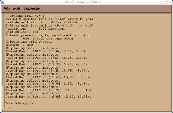
> addions 1PLC Na+ 8
This may take a few seconds to run. The output should look something like this.
Now we can try and save our prmtop and inpcrd files. At this point we should find that xleap cannot find the type CU or SM.
> saveamberparm 1PLC 1PLC.prmtop 1PLC.inpcrd
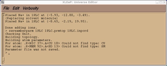
This is to be expected since CU and SM were atoms types that we made up that currently don't exist in the standard PARM99 force field. If you check our 1PLC unit you should also find, along with a large number of close contacts due to the solvation, a number of missing parameters all corresponding to the new CU and SM atom types.
> check 1PLC
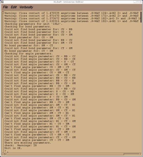
So, before we can go any further we need to add all of these parameters to the AMBER force field. Before we quit xleap however we shall save a 1PLC library file so that we don't have to repeat all of the steps we did above. We can just reload the library file.
> saveoff 1PLC 1PLC.lib
Here it is: 1PLC.lib
In order to introduce the new parameters we have two options. We can modify the main force field files or we can create an frcmod file with the changes specific to this project. The second option is a much better choice since modifying the main files could lead to clashes with other people who use the same installation. Creating a set of parameters is a bit of an art, since one is often faced with unknown parameters (such as force constants for copper to its ligands as in this example). The purpose of this tutorial is simply to cover the mechanics of running AMBER and so I provide you all of the parameters below. Note, these are for tutorial purposes only, I make no claims about the validity or appropriateness of these parameters. There are a number of articles in the literature about parameter estimation, and users are encouraged to consult them when faced with unusual chemical environments. A starting point is section 12.1 of the AMBER 8 manual entitled Parameter Development.
Here is the frcmod file I have created for plastocyanin:
# modifications to force field for poplar plastocyanin MASS SM 32.06 CU 65.36 BOND NB-CU 70.000 2.05000 #kludge by JRS CU-S 70.000 2.10000 #kludge by JRS CU-SM 70.000 2.90000 #for pcy CT-SM 222.000 1.81000 #met(aa) ANGLE CU-NB-CV 50.000 126.700 #JRS estimate CU-NB-CR 50.000 126.700 #JRS estimate CU-NB-CP 50.000 126.700 #JRS estimate CU-NB-CC 50.000 126.700 #JRS estimate CU-SM-CT 50.000 120.000 #JRS estimate CU-S -CT 50.000 120.000 #JRS estimate CU-S -C2 50.000 120.000 #JRS estimate CU-S -C3 50.000 120.000 #JRS estimate NB-CU-NB 10.000 110.000 #dac estimate NB-CU-SM 10.000 110.000 #dac estimate NB-CU-S 10.000 110.000 #dac estimate SM-CU-S 10.000 110.000 #dac estimate CU-SM-CT 50.000 120.000 #JRS estimate CT-CT-SM 50.000 114.700 #met(aa) HC-CT-SM 35.000 109.500 H1-CT-SM 35.000 109.500 CT-SM-CT 62.000 98.900 #MET(OL) DIHE X -NB-CU-X 1 0.000 180.000 3.000 X -CU-SM-X 1 0.000 180.000 3.000 X -CU-S -X 1 0.000 180.000 3.000 X -CT-SM-X 3 1.000 0.000 3.000 NONBON CU 2.20 0.200 SM 2.00 0.200 |
Anything with a # in front of it is a comment. As you can see we specify the mass, missing bonds, angle and dihedrals as well as VDW parameters.
We can now load this file into xleap and it will add all of these parameters to the PARM99 force field we selected.
$AMBERHOME/exe/xleap -s -f $AMBERHOME/dat/leap/cmd/leaprc.ff99
> loadamberparams plc.frcmod
> loadoff 1PLC.lib
We should now be able to create our topology and coordinate files.
> saveamberparm 1PLC 1PLC.prmtop 1PLC.inpcrd
Here are the files: 1PLC.prmtop, 1PLC.inpcrd
If you wish to look at the starting structure in vmd we can use ambpdb to create a pdb file for us:
$AMBERHOME/exe/ambpdb -p 1PLC.prmtop < 1PLC.inpcrd > 1PLC.inpcrd.pdb
Here it is: 1PLC.inpcrd.pdb
We could now use these files to run plastocyanin simulations. You can try this yourself if you want. Just remember that this is in explicit solvent and a peridiodic box so you use periodic boundary conditions. You will also need to minimise the system initially to remove bad contacts. I would then heat it over 20ps from 0 to 300K with constant volume periodic boundaries before moving to a long equilibration at 300 K with constant pressure.
(Note: These tutorials are meant to provide
illustrative examples of how to use the AMBER software suite to carry out
simulations that can be run on a simple workstation in a reasonable period of
time. They do not necessarily provide the optimal choice of parameters or
methods for the particular application area.)
Copyright Ross Walker 2008