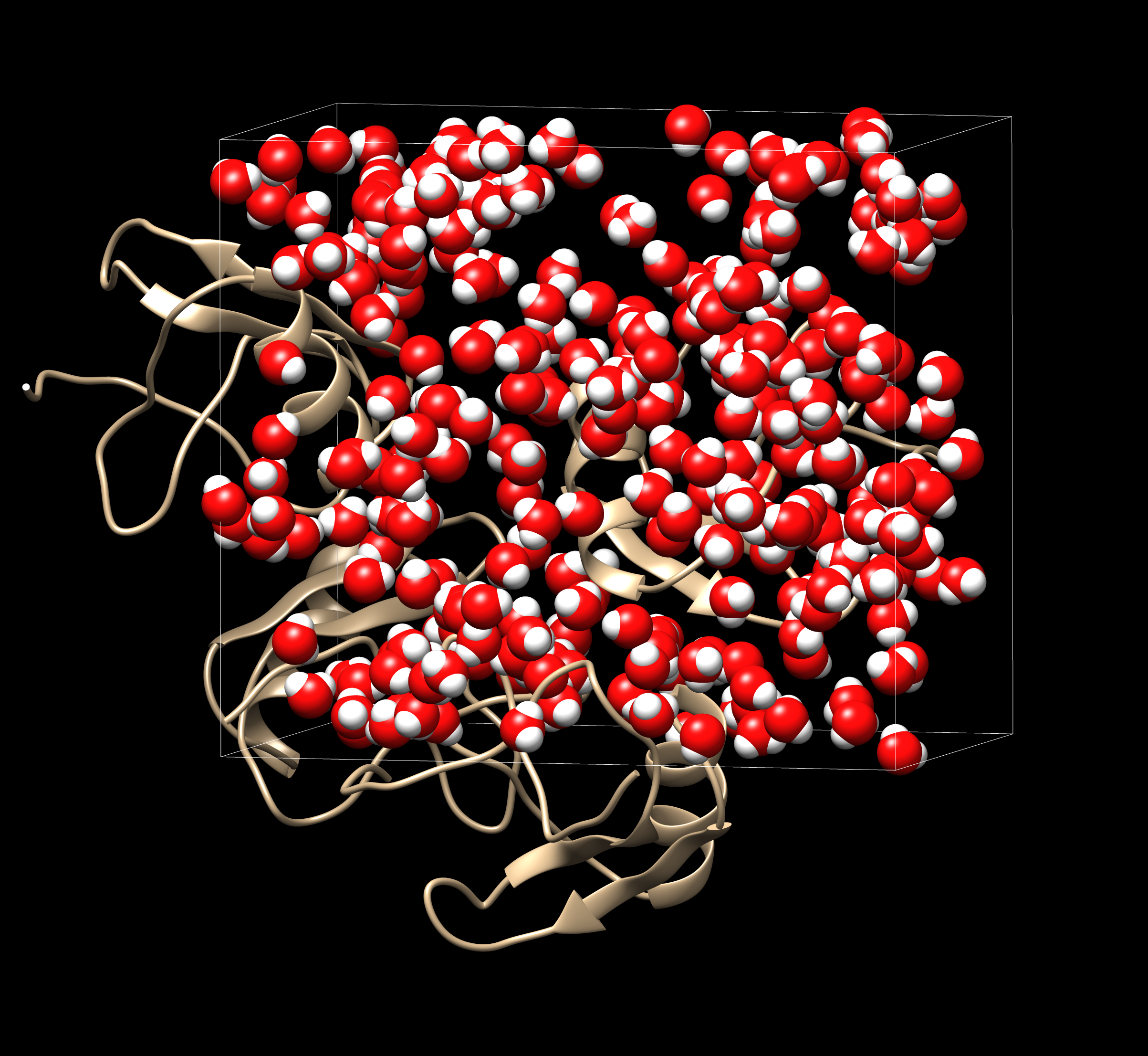
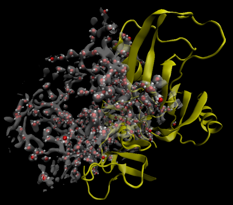
Placing waters and ions using 3D-RISM and MOFT

By David Case and George Giambasu

The output of this tutorial: water molecules whose placement in a crystal is based on a 3D-RISM calculation

Introduction

This tutorial demonstrates how to compute the solvent density around a protein (in this case a protein in a crystal lattice), and to place discrete water molecules or ions into the most favorable locations. It is based on 3D-RISM calculations (to get the solvent density distribution) and MOFT (to find optimal locations and place water molecules).

The basic outline of this tutorial is as follows:

Running a 3D-RISM calculation
Running metatwist to carry out a Laplacian analysis of the density
Placing discrete water molecules at the centers of negative Laplacian regions

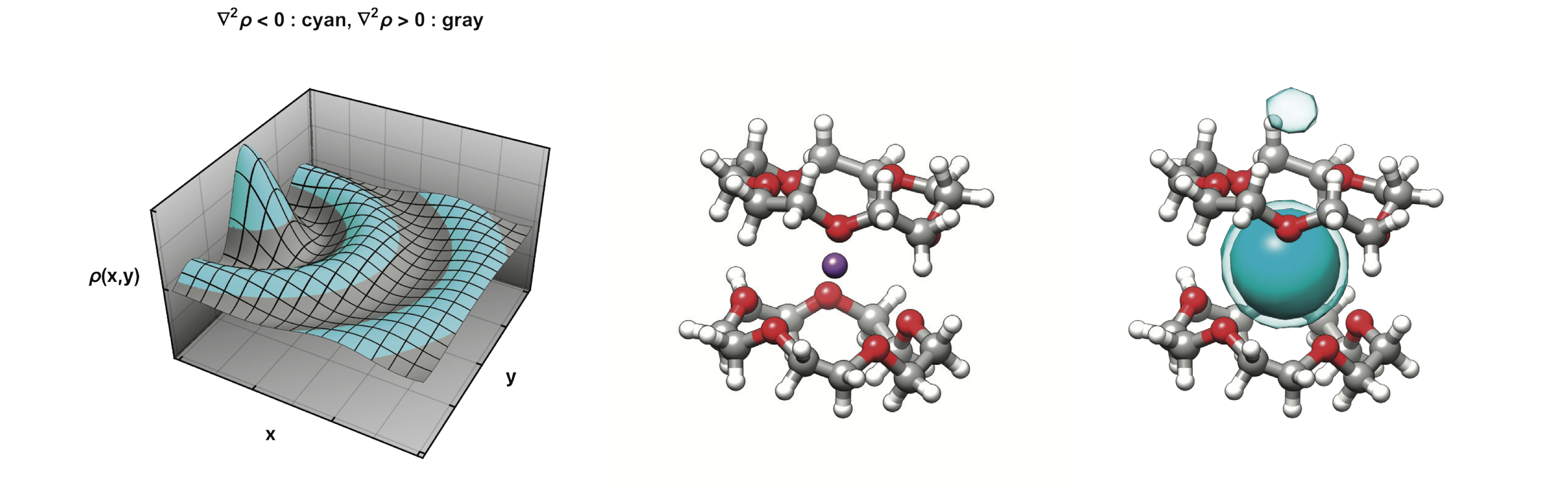
The basic reference here is Chapter 37 of the Amber 2019 Reference Manual, which gives more background and details than we can give here. But in brief, experience shows that a pre-conditioning using kernels that smooth out small local variations in the density can help eliminate false positives. Here we will apply the Laplacian mapping on the density convolution with a 3D Gaussian which can be carried out in a single step by a convolution with a Laplacian of a Gaussian kernel. Local (negative) minima of the Laplacian can be used to map locally concentrated regions of a density distribution. The basic idea is illustrated here:

(Left) The negative Laplacian (cyan) can be used to map locally concentrated regions of a density distribution; (Middle) A bis-crown ether (shown as CPK) binding mode to K+ (violet sphere) determined using density distributions obtained using RISM and located using Laplacian mapping in MoFT; (Right) Two level sets of the Laplacian of the K+ distribution, one using a threshold (see documentation) of 0.1 (solid cyan) and the other using a threshold of 0.01 (semi-transparent cyan).

Section 1: Running 3D-RISM

We start with pre-prepared prmtop and inpcrd files for a unit cell of the PDB code 1aho, which is a small scorpion toxin protein:

Here is the sander input (mdin.rism file) to run the 3D-RISM calculation:

single-point 3D-RISM calculation using the sander interface
&cntrl
ntx=1, nstlim=0, irism=1,
/
&rism
periodic='pme',
closure='kh', tolerance=1e-6,
grdspc=0.35,0.35,0.35, centering=0,
mdiis_del=0.4, mdiis_nvec=20, maxstep=5000, mdiis_restart=50,
solvcut=9.0,
verbose=2, npropagate=0,
apply_rism_force=0,
volfmt='dx', ntwrism=1,
/

and the corresponding arguments to sander:

sander -O -i mdin.rism -o 1aho.kh.r3d \
-p 1aho.parm7 -c 1aho.rst7 -xvv cSPCE_kh.xvv -guv 1aho.kh

Note that in this example, we are just doing a simple calculation with the KH closure and pure water. For more realistic simulations, one would use a higher closure (such as PSE3), and salt-water as a solvent.

If we use VMD (Chimera would also be fine) to visualize the DX map file 1aho.kh.O.0.dx, we would get a distribution that looks like this: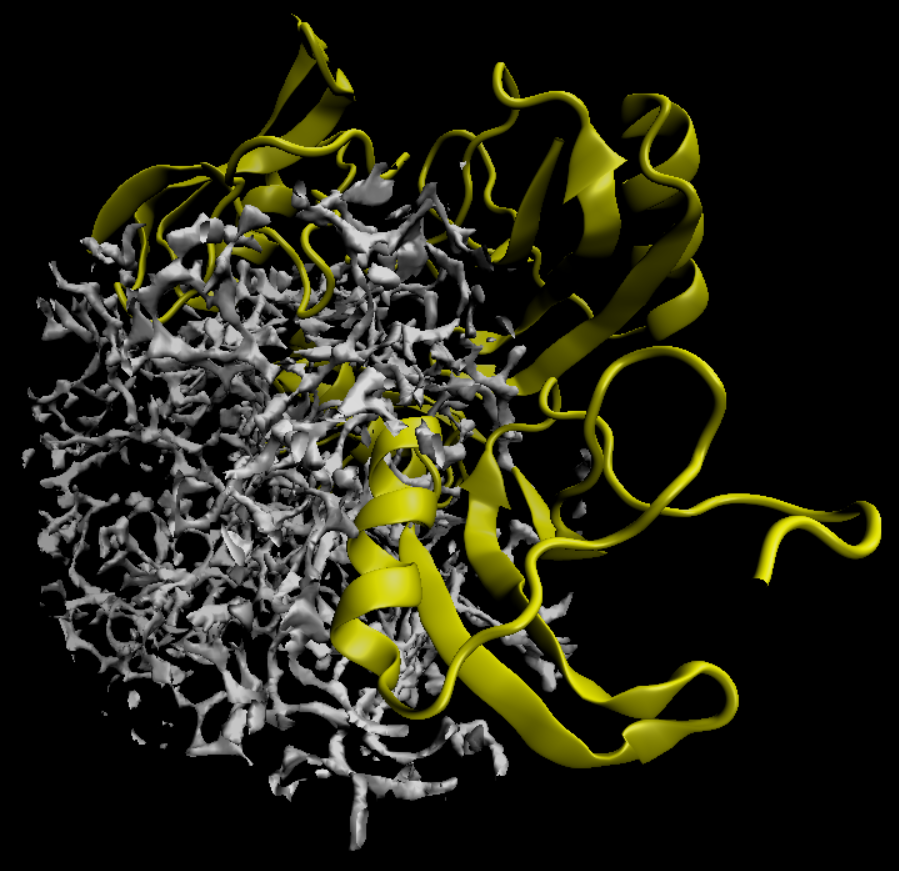

Visualization (using VMD) of the oxygen atom density in the 1aho unit cell. A yellow cartoon is used to show the location of the protein (pdb file) chains.

The "problem" with this representation is that it is difficult to see where waters are most likely to be found. We could try to search for the most positive densities and place water molecules at those points, but there are many local maxima, and they cannot all be occupied by waters. In the next section, we discuss a better way of representing the density.

Section 2: Running metatwist to carry out a Laplacian analysis of the density

The metatwist program will compute the Laplacian of the density, rather than just its value. Here are the commands that will do this:

metatwist --dx 1aho.kh.O.0.dx --species O \
--convolve 4 --sigma 1.0 --odx 1aho.kh.O.dx > 1aho.lp

The Laplacian density now looks like this:

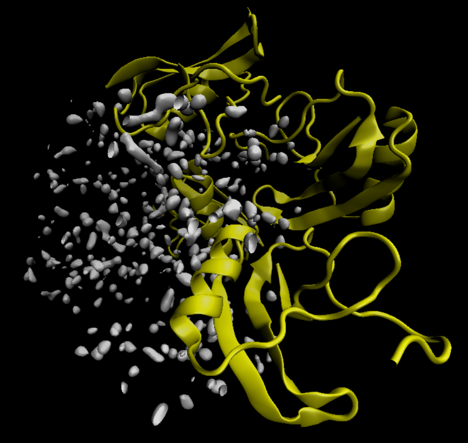
Visualization (using VMD) of the Laplacian negative values for oxygen atom density in the 1aho unit cell. A yellow cartoon is used to show the location of the protein chains.

Note that the most favorable regions are now much easier to identify, and a separated from one other. An algorithm can now find the centers of these "blobs", and place water molecules there>

Section 3: Place water molecules at the centers of the negative Laplacians

There are two pretty simple steps here. First, we use metatwist to place an oxygen at the center of each blob:

metatwist --dx 1aho.kh.O.0.dx \
--ldx 1aho.kh.O.dx --map blobsper \
--species O WAT --bulk 55.55 --threshold 0.5 > 1aho.blobs

This will create a 1aho.kh.O.0-1aho.kh.O-blobs-centroid.pdb file. It can be renamed by running

grep -v TER 1aho.kh.O.0-1aho.kh.O-blobs-centroid.pdb > wats.pdb

Finally, we use the gwh (Guess Water Hydrogens) code to add hydrogens, optimizing hydrogen bonding with the protein or with neighboring water molecules. Firstly it will be created a copy of 1aho.amber.pdb file with the name 1aho.wat.pdb:

sed 's/END/TER/' 1aho.amber.pdb > 1aho.wat.pdb

Then, the oxigens are added and hydrogens guessed by running:

gwh -p 1aho.parm7 -w wats.pdb < 1aho.amber.pdb >> 1aho.wat.pdb 2>> 1aho.blobs

The resulting water distribution is shown at the top of the tutorial. Visualizing this file along with the Laplacian, it is possible to see the water molecules located at the center of the blobs, as bellow:

Visualization (using VMD) of the water molecules inside the Laplacian negative values bobs. A yellow cartoon is used to show the location of the protein chains.

A complete script to automate the process is in the file run_rism_moft.