Amber Advanced Workshop - Tutorial 5 - Nudged Elastic Band - Section 5: Simulated Annealing and Equilibration

(Note: These tutorials are meant to provide illustrative examples of how to use the AMBER software suite to carry out simulations that can be run on a simple workstation in a reasonable period of time. They do not necessarily provide the optimal choice of parameters or methods for the particular application area.)
Copyright Ross Walker 2006

The Nudged Elastic Band Approach to Finding the Lowest Energy
Pathway Between two States

We will now run 100ps of MD at 300K with a much bigger spring constant. This will allow the structures to explore the energy landscape. At the same time we should be able to increase the time step to 1 fs now that we have successfully heated the system to 300 K and allowed it to relax slightly. Since we are only really going to be interested in the overall pathway, rather than the dynamics as we would be with a regular MD simulation I will set the mdcrd frequency to once every 5,000 steps (ntwx=5000). This allows us to avoid using too much disk space for a trajectory file we won't be using. We could turn of trajectory writing altogether but I like to have it write to the trajectory file occasionally as it can help in locating problems if things go wrong.

md-ala-neb_300K_equil.in

100ps NEB ALA-ALA equilibration
 &cntrl
  imin = 0, irest = 1, ntx=5,
  ntc=1, ntf=1,
  ntpr=1000, ntwx=5000,
  ntb = 0, cut = 999.0, rgbmax=999.0,
  igb = 1, saltcon=0.2,
  nstlim = 100000, nscm= 0,
  dt = 0.001,
  ntt = 3, gamma_ln=1000.0,
  temp0=300,
  ineb = 1,skmin = 50,skmax = 50
 /

We can now run this stage of MD using the sander.PIMD executable (This will take about 11 minutes to run on a single processor of a Pentium-D 3.2GHz Machine):

$AMBERHOME/exe/sander.PIMD -O -i md-ala-neb_300K_equil.in -o md-ala-neb_300K_equil.out -p neb.prmtop -c md-ala-neb-smallk_1.rst -r md-ala-neb_300K_equil.rst -x md-ala-neb_300K_equil.mdcrd

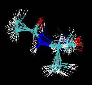
If you look at the output from this run you should observe that the structure with the highest energy changes during the simulation. This shows we are successfully exploring the energy surface. Open the mdcrd file in vmd (unzip it first). You should note that as this MD run progresses the structures gradually cover more of the conformational change.

The next step is to run a simulated annealing run. Here we shall use the NMR restraints option again to control the value of temp0 during the run. We will run a total of 300ps of MD (this should be sufficient for our small system) with the following temperature profile:

Note, as we will be heating to 500K it is necessary to reduce the time step to 0.5fs. This is because at these higher temperatures a 1fs time step without shake would cause instabilities. This annealing protocol is probably overkill for such a small system but it serves to illustrate how to do it.

md-ala-neb_anneal.in

300ps NEB ALA-ALA simulated annealing
 &cntrl
  imin = 0, irest = 1, ntx=5,
  ntc=1, ntf=1,
  ntpr=500, ntwx=10000,
  ntb = 0, cut = 999.0, rgbmax=999.0,
  igb = 1, saltcon=0.2,
  nstlim = 600000, nscm= 0,
  dt = 0.0005,
  ntt = 3, gamma_ln=1000.0,
  temp0=300,
  ineb = 1,skmin = 50,skmax = 50,
  nmropt=1
 /
 &wt type='TEMP0', istep1=0,istep2=100000,
   value1=300.0, value2=400.0
 /
 &wt type='TEMP0', istep1=100001,istep2=200000,
   value1=400.0, value2=400.0
 /
 &wt type='TEMP0', istep1=200001,istep2=300000,
   value1=400.0, value2=500.0
 /
 &wt type='TEMP0', istep1=300001,istep2=400000,
   value1=500.0, value2=500.0
 /
 &wt type='TEMP0', istep1=400001,istep2=500000,
   value1=500.0, value2=300.0
 /
 &wt type='TEMP0', istep1=500001,istep2=600000,
   value1=300.0, value2=300.0
 /
 &wt type='END'
 /

We can now run this simulated annealing protocol using the sander.PIMD executable (This will take about 1 hour to run on a single processor of a Pentium-D 3.2GHz Machine):

$AMBERHOME/exe/sander.PIMD -O -i md-ala-neb_anneal.in -o md-ala-neb_anneal.out -p neb.prmtop -c md-ala-neb_300K_equil.rst -r md-ala-neb_anneal.rst -x md-ala-neb_anneal.mdcrd

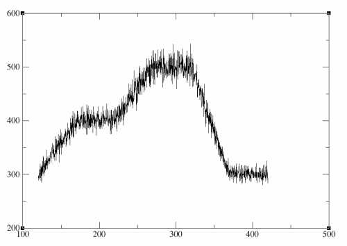
Before we proceed to the next stage and cool the system down so that it freezes out along the low energy pathway we should quickly check that the temperature profile we got from our simulated annealing run is what we expected. Here I will use grep to extract every line in the output file that contains the word NSTEP. I then 'pipe' this to awk which I use to extract only the 6th and 9th columns from each of those lines (these are the numerical values immediately after TIME = and TEMP =) and I write this to a file called temp_profile.dat. I have deleted the last two lines of this file as these two points refer to the RMS and average values. You can then plot this with whichever graphing program you like. As this is just a quick check that things proceeded okay I will use xmgrace:

As you can see below everything looks okay, the degree of fluctuations at the end of the trajectory, when we have cooled back down to 300 K, are roughly the same as those at the beginning of the trajectory and there are no sudden jumps in the temperature so everything looks good. You could try repeating the above simulation at 1 fs if you want and you will likely see that there are large jumps in the temperature and that after cooling back to 300 K at the end of the trajectory the temperature is still very unstable.