What is Jupyter notebook?
Direct introduction and figure from Jupyter notebook website:
"The Jupyter Notebook is a web application that allows you to create and share documents that contain live code, equations, visualizations and explanatory text. Uses include: data cleaning and transformation, numerical simulation, statistical modeling, machine learning and much more."
<img src="images/jupyterpreview.png", width=500>
What is pytraj?
pytraj is a Python package binding to the popular cpptraj program. pytraj is written do extend the flexibility of cpptraj and to expose cpptraj's functionality to Python's ecosystem, such as numpy, pandas, matplotlib, ...
What can you learn from this tutorial
Use Jupyter notebook for interactive data exploration
Use pytraj to perform basis analysis such loading files to memory and do computing RMSD
Use matplotlib and pandas for analyzing output from pytraj
Requirement
- AmberTools >= 16
- If you allow AMBER to install Python distribution from Miniconda, you have most needed packages (except pandas) for this tutorial.
- If not, you need to install (either using
piporconda)- matplotlib
- jupyter notebook
- Install pandas:
amber.conda install pandas
- You know how to use Linux command line. If not, please check basic AMBER tutorial
Download required trajectories, topology
All files used in this tutorial, including this notebook, is here: tutorial_files.zip
- Download it, then
mkdir tutorial
cd tutorial
unzip ../tutorial_files.zip
Start notebook
$ amber.jupyter notebook
(or jupyter notebook if you did not allow AMBER to install Miniconda)
- You should expect to see a blank directory (or with a list of files)
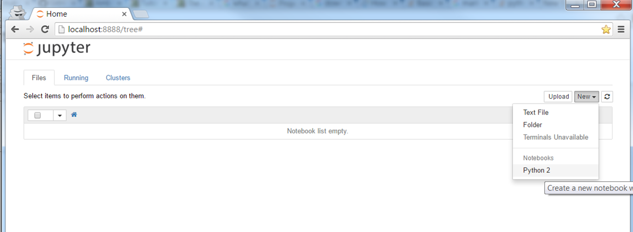
Choose New --> Python 2 (or Python 3, depending on which version you're using)
You should expect to see
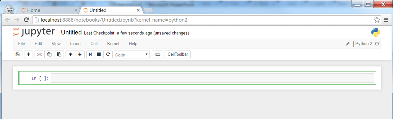
How to follow this tutorial? Copy and paste each command in this tutorial to the notebook, hit "Shift-Enter" to run and to create new Cell. Check Tips in the end of this tutorial for useful commands.
If you want to use the notebook remotely (run it in your remote cluster and view it in your desktop), please check remote notebook tutorial
Note: This tutorial is written in the Jupyter notebook, so you can download and run it too.
Load trajectory to memory
from __future__ import print_function
import warnings
warnings.filterwarnings("ignore", category=DeprecationWarning) # avoid warning message to make the notebook nicer

import pytraj as pt

traj = pt.load('data/trpzip2.gb.nc', top='data/trpzip2.ff10.mbondi.parm7')
Get some basic information about the trajectory
print(traj)
Computing RMSD, using 1st frame as reference
In this case we are computing mass-weighted RMSD, using all non-hydrogen atoms in residues 1 to 13
data_rmsd_first = pt.rmsd(traj, ref=0, mask=":1-13&!@H*")

print(data_rmsd_first)
Using matplotlib to plot
%matplotlib inline

from matplotlib import pyplot as plt

plt.plot(data_rmsd_first)
plt.xlabel('Frame')
plt.ylabel('RMSD (Angstrom)')

Loading reference structure
In this case, we are loading the NMR structure for trpzip2
# we can reuse loaded topology from `traj`
ref = pt.load('data/trpzip2.1LE1.1.rst7', top=traj.top)
print(ref)
Computing RMSD to a Reference
data_rmsd_ref = pt.rmsd(traj, ref=ref, mask=":1-13&!@H*")
print(data_rmsd_ref)
Plotting two RMSDs
We can plot rmsd to 1st frame (previously calculated) and rmsd to reference (NMR)
plt.plot(data_rmsd_first, label='to first')
plt.plot(data_rmsd_ref, label='to NMR')
plt.xlabel('Frame')
plt.ylabel('RMSD (Angstrom)')
plt.legend()

Computing pairwise RMSD for specific snapshots
# compute pairwise RMSD for first 50 snapshots and skip every 10 frames
mat = pt.pairwise_rmsd(traj, mask=":1-13&!@H*", frame_indices=range(0, 500, 10))
print(mat)
plt.imshow(mat, cmap='jet')
plt.xlabel('Frame')
plt.ylabel('Frame')
plt.colorbar()

Computing dihedral angles
In this case, we are computing phi and psi angle for residues 2 to 12. We tell pytraj to convert raw data to pandas's DataFrame to better visualization in notebook
phipsi = pt.multidihedral(traj, resrange='1-12', dihedral_types="phi psi", dtype='dataframe')
Pretty display data
In this case, we only display a part of the data
phipsi[['phi_4', 'psi_4', 'phi_5', 'psi_5']].head(5)
Getting some basic info
phipsi[['phi_4', 'psi_4', 'phi_5', 'psi_5']].describe()
Plotting dihedral
In this case, we are plotting Psi dihedral for residue 4 (TRP)
plt.plot(phipsi['psi_8'], '-bo', markersize=3, linewidth=0)
plt.xlabel('Frame')
plt.ylabel('Phi4')

Get some information about the structure
top = traj.top

for residue in top.residues:
    # Note: In python, 0-based index is used.
    # For example: SER0 should be first residue
    print(residue)
list(traj.top.atoms)[:10]
Tips
- Run bash command: Use !
! echo Hello
How to run this notebook?
- Run all commands: Cell -> Run All
- Run each Cell: Ctrl-Enter
- Run each Cell and jump to next Cell: Shift-Enter
- How to save all commands to Python script: Choose File -> Download as -> Python (.py)
- How to save figures in this notebook: Right click and choose Save image as (or similiar command)
- More info? Choose Help -> Keyboard Shortcuts
See also
If you would like to learn more about pytraj, please see unofficial AMBER tutorials for pytraj in pytraj website