(Note: These tutorials are meant to provide
illustrative examples of how to use the AMBER software suite to carry out
simulations that can be run on a simple workstation in a reasonable period of
time. They do not necessarily provide the optimal choice of parameters or
methods for the particular application area.)
Copyright Ross Walker 2004
AMBER ADVANCED WORKSHOP
TUTORIAL A5 - SECTION 4
The Nudged Elastic Band Approach to Finding the Lowest
Energy
Pathway Between two States
By Ross Walker
4. Heating the System
The first stage of our NEB MD simulation will be to carefully heat the system up. Note, if you tried to run normal MD with the neb.prmtop and neb.inpcrd files your system would blow up quite spectacularly since these files contain two sets of 15 structures all on top of each other. The electrostatic and VDW repulsion would be infinite on the first step. In the NEB method though the individual molecules never see each other. They only feel a force due to the two springs connecting them to their nearest neightbours.
We are now ready to run MD on our system. The first thing we should do is allow our system to warm up from 0 to 300K. We need to be very careful here though as our initial spring forces will be very large. Hence we do this stage with a small spring constant. Here is the input file we will use, we will run 20ps of MD with a 0.5fs time step (nstlim=40000, dt=0.0005). The half femtosecond time step is probably overkill but it will improve the chances of our simulation remaining stable early on. We will not be using shake to constrain hydrogens in this simulation since the interesting region of the pathway will involve changes in hydrogen bond lengths (ntc=1, ntf=1). This means that even once we have our system equilibrated we will be restricted to a time step of at a maximum 1 fs. Since the coordinates of the end points are fixed in Cartesian space in NEB and the intervening structures cannot move far due to the springs there is no need to recenter the coordinates every few hundred steps so we turn this off (NSCM=0). We will use generalised born for the implicit solvent with a sodium chloride salt concentration of 0.2M (igb=1, saltcon=0.2). The system is small enough here that I will avoid any issues with nonbonded cutoffs and truncated Born radii calculations by setting these to 999.0 angstroms (cut=999.0, rgbmax=999.0). This has the effect of turning off any nonbond cutoff. The NEB specific options are on the last line (ineb=1 [turn on neb], skmin=10, skmax=10 [spring constants]. We start here with relatively small spring constants of 10 KCal/mol/A2. We will increase this value later once the system has begun to equilibrate.
For temperature regulation we use the langevin thermostat (ntt=3) and we will use a very high collision rate of 1000 ps-1 (gamma_ln=1000). This would be extremely high for a regular MD simulation where values of around 5.0 are more appropriate. However, in NEB we are not interested in the actual dynamics, we simply want to ensure that our system explores as much phase space as possible before we cool it back down to 0 K and so we use a high collision rate to ensure rapid uniform heating, give the system some viscosity and improve the stability. Without the strong thermostat, the calculation would become unstable because the periodic motions involving the springs (and the truncation of the forces according to the path tangent) would blow the system apart. Thus it is essential to use very very large values of gamma_ln with NEB simulations.
The large value of gamma_ln would normally mean that our system would heat up to the value of temp0 very rapidly, within a few pico-seconds. This could cause instabilities in the simulation and so we will use NMR weight restraints (nmropt=1) to linearly increase the value of temp0 from 0.0 to 300.0 K over 35,000 steps of the 40000 step simulation (istep1=0,istep2=35000, value1=0.0, value2=300.0). This means that at step 0 the value of the target temperature (temp0) will be 0.0 K. At step 5,000 it will be 42.86 K, at 10,000 it will be 85.72 K, by 20,000 it will be 171.44 K and by 35,000 it will be at 300.0 K. It will then remain at 300.0 K until the end of our 40,000 step run. In this way our system should heat up in a controlled fashion.
Alanine NEB initial MD with small K &cntrl imin = 0, irest = 0, ntc=1, ntf=1, ntpr=50, ntwx=500, ntb = 0, cut = 999.0, rgbmax=999.0, igb = 1, saltcon=0.2, nstlim = 40000, nscm= 0, dt = 0.0005, ntt = 3, gamma_ln=1000.0, tempi=0, temp0=300, ineb = 1,skmin = 10,skmax = 10, nmropt=1 / &wt type='TEMP0', istep1=0,istep2=35000, value1=0.0, value2=300.0 / &wt type='END' / |
We can now run this MD using the AMBER v9 Sander.PIMD executable (sander.PIMD.MPI if we want to run the simulation in parallel). This will take about 4.5 minutes to run on a single processor of a Pentium-D 3.2GHz Machine:
$AMBERHOME/exe/sander.PIMD -O -i md-ala-neb-smallk_1.in -o md-ala-neb-smallk_1.out -p neb.prmtop -c neb.inpcrd -r md-ala-neb-smallk_1.rst -x md-ala-neb-smallk_1.mdcrd
Input Files: md-ala-neb-smallk_1.in,
neb.prmtop,
neb.inpcrd
Output Files: md-ala-neb-smallk_1.out,
md-ala-neb-smallk_1.rst,
md-ala-neb-smallk_1.mdcrd
Take a look at the output file. It looks just like a normal MD except that you now have the energy of each of the 30 replicates listed. This is the energy of each one as it moves along the potential energy surface. You also see the total energy of the replicates. The lowest energy pathway should be the one for which this sum is the smallest. Thus if we perform simulated annealing calculations and obtain several pathways we can compare the overall sum from each pathway. Take a quick look at the output file and check that the simulation looks stable, i.e. the temperature changes as we expect, slowly increasing to 300.0 K and then oscillating around this value. Any huge temperature jumps are signs of problems with our simulation, poor starting structure, poor choice of simulation options etc. You should also take a look at the replicate energies. These show the potential energy of each replica on the pathway. The most important thing to check at this stage is that on step 0 the first 15 have the same energy, that of the beginning of the pathway and the last 15 have a different but identical energy, that of the end of the pathway. If this is not the case then something is wrong with the neb.prmtop and neb.inpcrd files.
 NSTEP =        0   TIME(PS) =       0.000  TEMP(K) =     0.00  PRESS =     0.0
 Etot   =      -972.8504  EKtot   =         0.0000  EPtot      =      -992.5236
 BOND   =        17.6624  ANGLE   =        54.1617  DIHED      =       210.8264
 1-4 NB =        88.0044  1-4 EEL =      1326.1645  VDWAALS    =       -49.1867
 EELEC  =     -2086.7405  EGB     =      -553.4159  RESTRAINT  =         0.0000
NEB replicate breakdown:
Energy for replicate   1 =      -33.7654
Energy for replicate   2 =      -33.7654
Energy for replicate   3 =      -33.7654
Energy for replicate   4 =      -33.7654
Energy for replicate   5 =      -33.7654
Energy for replicate   6 =      -33.7654
Energy for replicate   7 =      -33.7654
Energy for replicate   8 =      -33.7654
Energy for replicate   9 =      -33.7654
Energy for replicate  10 =      -33.7654
Energy for replicate  11 =      -33.7654
Energy for replicate  12 =      -33.7654
Energy for replicate  13 =      -33.7654
Energy for replicate  14 =      -33.7654
Energy for replicate  15 =      -33.7654
Energy for replicate  16 =      -32.4029
Energy for replicate  17 =      -32.4029
Energy for replicate  18 =      -32.4029
Energy for replicate  19 =      -32.4029
Energy for replicate  20 =      -32.4029
Energy for replicate  21 =      -32.4029
Energy for replicate  22 =      -32.4029
Energy for replicate  23 =      -32.4029
Energy for replicate  24 =      -32.4029
Energy for replicate  25 =      -32.4029
Energy for replicate  26 =      -32.4029
Energy for replicate  27 =      -32.4029
Energy for replicate  28 =      -32.4029
Energy for replicate  29 =      -32.4029
Energy for replicate  30 =      -32.4029
Total Energy of replicates =     -992.5236
NEB RMS =      1.547934
 ------------------------------------------------------------------------------
NMR restraints: Bond = 0.000 Angle = 0.000 Torsion = 0.000 =============================================================================== NSTEP = 50 TIME(PS) = 0.025 TEMP(K) = 0.98 PRESS = 0.0 Etot = -979.3091 EKtot = 1.9186 EPtot = -981.2277 BOND = 24.1932 ANGLE = 58.2929 DIHED = 212.3182 1-4 NB = 88.2867 1-4 EEL = 1324.0833 VDWAALS = -49.3134 EELEC = -2087.5767 EGB = -551.5120 RESTRAINT = 0.0000 NEB replicate breakdown: Energy for replicate 1 = -33.7654 Energy for replicate 2 = -33.7510 Energy for replicate 3 = -33.7567 Energy for replicate 4 = -33.7551 Energy for replicate 5 = -33.7535 Energy for replicate 6 = -33.7561 Energy for replicate 7 = -33.7562 Energy for replicate 8 = -33.7512 Energy for replicate 9 = -33.7539 Energy for replicate 10 = -33.7550 Energy for replicate 11 = -33.7589 Energy for replicate 12 = -33.7547 Energy for replicate 13 = -33.7536 Energy for replicate 14 = -33.7530 Energy for replicate 15 = -27.9942 Energy for replicate 16 = -27.1873 Energy for replicate 17 = -32.3828 Energy for replicate 18 = -32.3861 Energy for replicate 19 = -32.3918 Energy for replicate 20 = -32.3893 Energy for replicate 21 = -32.3946 Energy for replicate 22 = -32.3918 Energy for replicate 23 = -32.3902 Energy for replicate 24 = -32.3863 Energy for replicate 25 = -32.3904 Energy for replicate 26 = -32.3895 Energy for replicate 27 = -32.3935 Energy for replicate 28 = -32.3920 Energy for replicate 29 = -32.3908 Energy for replicate 30 = -32.4029 Total Energy of replicates = -981.2277 NEB RMS = 3.078592 ------------------------------------------------------------------------------ |
We have to do quite a bit of simulated annealing, however, to find the lowest pathway. We also need to increase the strength of our initial 'weak' spring constant.
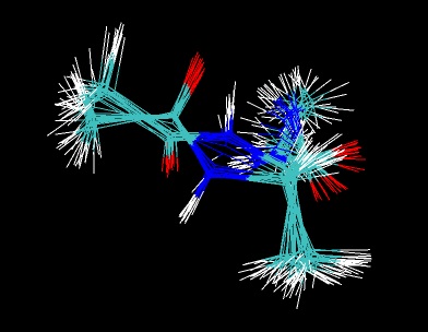
Before we move on though it is interesting to look at the mdcrd file in vmd. Here you will see all of the structures. Run VMD and load the neb.prmtop and the md-ala-neb-smallk_1.mdcrd file (note: I gzipped the mdcrd file to save space. Ensure you unzip it before loading it in VMD)

Notice how all the structures are still grouped around one of the starting structures. This is because our spring constant wasn't large enough to pull them over the hill between the two end points. It has removed some of the strain on the system however. We are now ready to move onto the next stage of the simulation where we will conduct the simulated annealing and equilibration.