What is NGLView?
NGLView is a viewer for molecular structures and trajectories in Jupyter notebook.
Requirement
- AmberTools >= 16
- If you allow AMBER to install Python distribution from Miniconda, you have most needed packages (except NGLView) for this tutorial.
- If not, you need to install (either using
piporconda)conda install jupyter notebook
- Install NGLView development version:
amber.conda install nglview -c bioconda - You know how to use Linux command line. If not, please check basic AMBER tutorial
- You know how to open a Jupyter notebook
How to follow this tutorial?
- Open notebook
amber.jupyter notebook notebook.ipynb # where notebook.ipynb is the name of this notebook Just copy and paste commands to your notebook, then hit "Ctrl-Enter"
Files: tutorial_files.zip
Example: View a single pdb file
import warnings
warnings.filterwarnings('ignore') # make the notebook nicer
from __future__ import print_function
import pytraj as pt
import nglview as nv
print("nglview version = {}".format(nv.__version__))
print("pytraj version = {}".format(pt.__version__))
traj = pt.load('data/wt1mg.pdb')
view = nv.show_pytraj(traj)
view
You should expect to see
view.render_image()
view._display_image()
from IPython.display import IFrame
IFrame(src="view.html", width=700, height=700)
Example: View an AMBER trajectory
traj2 = pt.load('data/DPDP.nc', 'data/DPDP.parm7')
# superpose to 1st frame, using only CA atoms
traj2.superpose(ref=0, mask='@CA')
view2 = nv.show_pytraj(traj2)
view2.clear_representations()
view2.add_representation('cartoon')
view2.add_representation('licorice', selection='not hydrogen')
view2
You should expect to see
view2.render_image()
view2._display_image()
Example: Load ccp4 data
# load pdb file
traj3 = pt.load('data/3pqr.pdb')
# create view
view3 = nv.show_pytraj(traj3)
# display
view3.center_view()
view3
# load ccp4 data
# use: view3._load_data
view3._load_data('data/3pqr.ccp4.gz')
# add representations for loaded data (model 1)
view3._clear_repr(component=1)
view3.add_surface(component=1, color='blue', wireframe=True, opacity=0.2, isolevel=3.)
After zooming in by mouse, you should expect to see
view3.render_image()
# need to call _display_image in different Cell
view3._display_image()
Example: Display Lipid Bilayer
# PDB file is from: http://www.ks.uiuc.edu/Training/Tutorials/science/membrane/
traj_lipid = pt.load('data/kcsa_popcwi.pdb')
print(traj_lipid)
view_lipid = nv.show_pytraj(traj_lipid)
view_lipid
view_lipid.clear_representations()
view_lipid.add_cartoon('protein')
view_lipid.add_licorice('TIP and not hydrogen', linewidth=1.)
view_lipid.add_licorice('not hydrogen', opacity=0.5)
view_lipid.orientation = [[-70.94550361812348, -23.54590217040876, -13.725642929758788],
[0.17341421016637665, 0.05082474596059873, -0.9835366576342925],
[-0.10400009155273438, 1.1669998168945312, -5.298999786376953],
[0, 0, 0]]
view_lipid.render_image()
view_lipid._display_image()
Render high quality image
NGLView is able to render high quality image for publication. You can call download_image(...) method.
# specify very high `factor` value to have better quality
# NGLView will render the current frame and download the image
# uncomment for rendering
# view3.parameters = dict(theme='light')
# view3.download_image(filename='my_image.png', factor=15, trim=True)
click here to see the rendered image
You can also use pytraj to analyze data - Example: compute DSSP
dssp_data = pt.dssp(traj2)
print('resdues = {}'.format(dssp_data[0]))
print('dssp = {}'.format(dssp_data[1]))
You can also use pytraj to make new trajectory and visualize it
Replicate cell
# load a trajectory with single frame
traj3 = pt.datafiles.load_tz2_ortho()[:1]
traj3
view3 = nv.show_pytraj(traj3)
view3.representations = []
view3
view3.add_representation('cartoon', selection='protein', color='blue')
view3.add_representation('line', selection='water')
traj4 = pt.replicate_cell(traj3, direction=('001', '111'))
traj4
view4 = nv.show_pytraj(traj4)
view4.representations = []
view4
view4.add_representation('cartoon', selection='protein', color='blue')
view4.add_representation('line', selection='water')
Click here if you want to see how to result looks like
view4.orientation = [[1.7307010437006827, 14.438547748522044, -72.27208013737686],
[-0.6887824733588872, 0.7139114858593536, 0.1261312600100375],
[-35.171499490737915, -41.96850076317787, -54.250999450683594],
[0, 0, 0]]
view4.render_image()
view4._display_image()
Example: Using two consoles for visualization
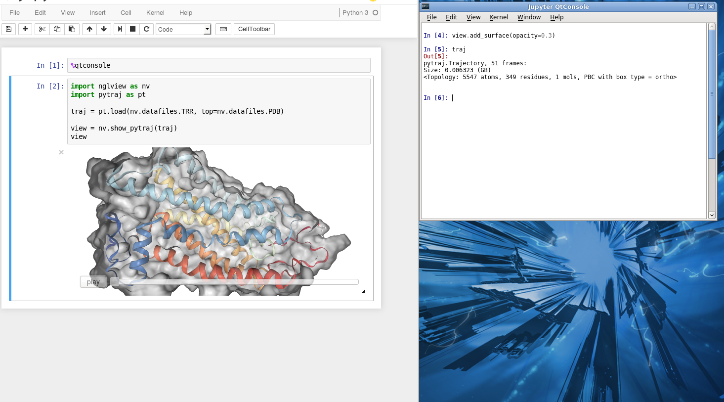
Sometimes it is more convinient to use two screens or two consoles, one for viewing protein and one for performing analysis (like VMD, PyMol, ...). You can also do that with Jupyter notebook.
First, open the notebook. In the first Cell (or your favorite Cell), enter:
%qtconsole # make sure to run the Cell
A new console will pop up. It share the same memory with the notebook. You can control the viewer by typing any command in this new console.

updated date
from time import gmtime, strftime
strftime("%Y-%m-%d", gmtime())