Computing the Short-Ranged Potential
The short-ranged potential, also known as the "direct space sum," is
conceptually the simplest part of PME. Simply loop over all particles i
and j, compute the minimum image distance between them, and if the
distance rij is within the cutoff, apply
kqiqj(1 -
erf(αrij))/rij to get the energy
contribution (differentiate to get the force--this part of the potential is
often splined for efficiency).
This is an ideal time to look at the Ewald coefficient, which to reiterate
is the inverse of the Gaussian charge spreading factor. The function
getalpha takes two arguments, the short-ranged potential cutoff
and the direct sum tolerance:
getalpha(8.0, 1.0e-5)

ans = 0.3486
Running that in a loop to generate multiple Gaussian charge spreading
factors shows a nearly linear relationship with the cutoff:
i = 0;
gspread = zeros(1,61);
for Lcut = 6.0:0.1:12.0, i = i+1; gspread(i) = 0.5/getalpha(Lcut, 1.0e-5); end
plot(6.0:0.1:12.0, gspread, 'r.', 'markersize', 24);
hold on;
i = 0;
for Lcut = 6.0:0.1:12.0, i = i+1; gspread(i) = 0.5/getalpha(Lcut, 5.0e-6); end
plot(6.0:0.1:12.0, gspread, 'k.', 'markersize', 24);
i = 0;
for Lcut = 6.0:0.1:12.0, i = i+1; gspread(i) = 0.5/getalpha(Lcut, 1.0e-6); end
plot(6.0:0.1:12.0, gspread, '.', 'color', [1.0 0.4 0.0], 'markersize', 24);
axis([6 12 1.0 2.4]);
daspect([4 1 1]);
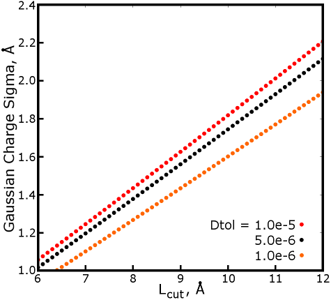
This is a useful result--for all practical values of the short-ranged cutoff
and direct sum tolerance, the Gaussian charge spreading factor is nearly
proportional to the cutoff. The ratio of the charge spreading factor to mesh
grid spacing is essential to precision in the reciprocal space part of the
calculation. For the default Amber interpolation method (4th order,
this will be explained in detail later), the charge spreading factor needs to
be about 1.5 times the mesh spacing to meet the short-ranged potential
precision imparted by a direct sum tolerance of 1.0e-5 (note how this matches a
spreading factor of 1.434Å to mesh spacings of close to but not exceeding
1.0Å). For a more expensive interpolation scheme (6th order),
the spreading factor can be as small as the 1.0 times the mesh spacing and
still provide a precise long-ranged potential calculation. That relationship
breaks down a bit for really large mesh spacings (⋝ 1.8Å), but it
is seldom worthwhile to extend the cutoff that far just to get a coarser
mesh.
While the short-ranged, "direct space" potential is conceptually simple, the
O(N2) problem arises again, and the code can be much more efficient
by testing only interactions that are likely to yield success on the cutoff
criterion. This is the origin of neighbor lists, hash tables,
neutral
territory methods, and multiple time steps to avoid recalculating the
tail of the electrostatic short-ranged potential, which is small and changes
slowly. The complexities introduced by all of these factors create the
preponderance of code devoted to direct space electrostatics in most modern
MD packages. The PME library contains pmeDirectBasicLoop.m for
the basic all-to-all particle-particle computation,
pmeDirectMidpointOrthog.m for the midpoint method, and
pmeDirectTowerPlate.m for the tower-plate method. While these
codes illustrate various distinct methods of performing the direct space
decomposition, none of them is highly optimized.
To run the direct space calculation as a standalone operation, we first need
a system: a four-column matrix containing coordinates and charges, [ X Y Z Q ],
plus a box size. Take the cubeions system in the
Tests/ folder. The dimensions array has only three elements, but
the box angles are then assumed to all be 90°. Any of the three functions
can then be used to calculate the forces on the particles:
load Tests/cubeions.mat
Lcut = 8.0;
dtol = 1.0e-5;
ewcoeff = getalpha(Lcut, dtol);
fbasic = pmeDirectBasicLoop(crdq, 0, gdim, ewcoeff, Lcut);
ftower = pmeDirectTowerPlate(crdq, 0, gdim, ewcoeff, Lcut);
fmidpt = pmeDirectMidpointOrthog(crdq, 0, gdim, ewcoeff, Lcut);
Even in Matlab, with all its clunky loops, it is evident that the methods
based on hash cells are faster than the all-to-all implementation, which is so
slow for systems of any significant size that it periodically prints progress
to the terminal to let users know that Matlab didn't hang. The differences in
forces will be below 1.0e-4 kcal/mol-Å, but not trivial due to splined
versus analytic computation of the short-ranged potential and also
non-associativity in floating-point addition.
A different exercise can illustrate how the Ewald coefficient / Gaussian
spreading factor controls the way in which Coulomb's law is split into short-
and long-ranged parts. Try re-calculating the forces using a different cutoff,
but the same Ewald coefficient.
Lcut = 8.0;
ewcoeff  = getalpha(Lcut, 1.0e-5);
fmidpt8  = pmeDirectMidpointOrthog(crdq, 0, gdim, ewcoeff, Lcut);
fmidpt9  = pmeDirectMidpointOrthog(crdq, 0, gdim, ewcoeff, Lcut + 1.0);
fmidpt10 = pmeDirectMidpointOrthog(crdq, 0, gdim, ewcoeff, Lcut + 2.0);
fmidpt12 = pmeDirectMidpointOrthog(crdq, 0, gdim, ewcoeff, Lcut + 4.0);
It is easy to check that forces in fmidpt8 and fmidpt9 may differ by up to a
hundredth of a kcal/mol-Å. Not a big deal, given the magnitudes of the
actual forces. As would be expected, fmidpt9 and fmidpt10 differ by much
less‐about an order of magnitude‐and fmidpt10 and fmidpt12 hardly
differ at all. The short-ranged potential and its gradients converge. But,
this is not an exercise that can be done with the sander or
pmemd programs--they calculate the Ewald coefficient given a
short-ranged cutoff and a direct sum tolerance, whereas here we have kept the
Ewald coefficient fixed and in effect driven down the direct sum tolerance with
increasingly long cutoffs, computing the sum beyond the original limit of
8Å. In the mdgx program, a niche application, it is
possible to set the Gaussian charge spreading factor explicitly, in which case
the direct sum tolerance will be determined based on the short-ranged cutoff.
We can emulate the behavior of the workhorse Amber MD engines as follows:
Lcut = 8.0;
ewcoeff  = getalpha(Lcut, 1.0e-5);
fmidpt8  = pmeDirectMidpointOrthog(crdq, 0, gdim, ewcoeff, Lcut);
Lcut = 9.0;
ewcoeff  = getalpha(Lcut, 1.0e-5);
fmidpt9  = pmeDirectMidpointOrthog(crdq, 0, gdim, ewcoeff, Lcut);
A simple comparison of the forces reveals that the two are markedly
different‐this is not because either is wrong, but rather the splitting
has changed, with the Gaussian charge spreading factor being 1.434Å in
the first case and 1.625Å in the second. We can use
getalpha with guess-and-check to determine what the direct sum
tolerance would need to be in order to match the original splitting:
0.5/getalpha(9.0, 5.0e-6) = 1.5597
0.5/getalpha(9.0, 2.0e-6) = 1.4840
0.5/getalpha(9.0, 1.0e-6) = 1.4334
0.5/getalpha(9.0, 1.1000e-6) - 0.5/getalpha(8.0, 1.0e-5) = 0.0059
0.5/getalpha(9.0, 1.0500e-6) - 0.5/getalpha(8.0, 1.0e-5) = 0.0026
0.5/getalpha(9.0, 1.0250e-6) - 0.5/getalpha(8.0, 1.0e-5) = 0.0009
0.5/getalpha(9.0, 1.0250e-6) - 0.5/getalpha(8.0, 1.0e-5) = 0.0009
0.5/getalpha(9.0, 1.0115e-6) - 0.5/getalpha(8.0, 1.0e-5) = 3.1969e-6
Extending the cutoff by 1.0Å allows us to converge the direct space
sum almost one order of magnitude more tightly while conserving the precision
of the reciprocal space sum.
Go to the next section
Go to the previous section
|


