


(Note: These tutorials are meant to provide
illustrative examples of how to use the AMBER software suite to carry out
simulations that can be run on a simple workstation in a reasonable period of
time. They do not necessarily provide the optimal choice of parameters or
methods for the particular application area.)
Copyright Jason Swails & T. Dwight McGee Jr 2013
Section 2: Preparing the system
This section describes the steps required to prepare the system you built in Section 1 for CpHMD simulations in Amber.
There are three general setup phases that come before the main production simulations (these are common with many other types of simulations):
- Minimize system to relax bad contacts (jump here)
- Heat the system slowly to the target temperature (jump here)
- Equilibrate the system at the target temperature (jump here)
Minimizing the system
The first stage is minimizing the protein. Because the charges and initial protonation states of the various titratable residues are defined in the cpin file, the minimization should be run with sander with constant pH specified.
The input file is shown below:
| min.mdin |
|
Minimization to prepare for constant pH MD &cntrl imin = 1, ! Turn on minimization igb = 2, ! Use the GB model CpHMD was parametrized for saltcon = 0.1, ! Use the salt conc. CpHMD was parametrized for maxcyc = 1000, ! Total number of minimization cycles icnstph = 1, ! Turn on constant pH ntcnstph = 100000, ! Never attempt to change prot. states cut = 1000.0, ! No cutoff ntr = 1, ! Turn on positional restraints restraint_wt = 10, ! 10 kcal/mol/A**2 restraint force constant restraintmask = '@CA,C,O,N' ! Restraints on the backbone atoms only / |
To run this simulation, we use the command:
mpiexec -n 4 sander.MPI -O -i min.mdin -p 4LYT.parm7 -c 4LYT.rst7 -o 4LYT.min.mdout -r 4LYT.min.rst7 -ref 4LYT.rst7 -cpin 4LYT.cpin
Because this is a large protein (1997 atoms) and GB simulations scale well up to a large number of processors, 4 cores on a standard desktop was used for this stage. At this point, you should get a restart (4LYT.min.rst7) and an output file (4LYT.min.mdout). At this stage, it is always a good idea to inspect the energies in your output file to make sure that the trend makes sense. mdout_analyzer.py is a nifty tool to help you quickly analyze data printed from sander or pmemd simulations.
To run this program, type 'mdout_analyzer.py 4LYT.min.mdout' and then select the term you wish to graph (ENERGY) and click 'Graph Them!'. Graphing the energies should look like:
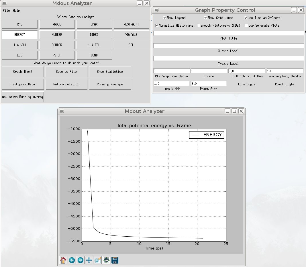
As we expect, the energy drops rapidly as the structure relaxes. We are now ready for dynamics. (As another note, it is never a bad idea to use VMD to inspect the structures to make sure they did not visibly blow apart during the calculation).
Heating the system
In this step, we will heat the system slowly up to 300 K, keeping restraints on the backbone atoms again. The input file is shown below:
| heat.mdin |
|
Implicit solvent constant pH initial heating mdin &cntrl imin=0, irest=0, ntx=1, ntpr=500, ntwx=500, nstlim=1000000, dt=0.002, ntt=3, tempi=10, temp0=300, tautp=2.0, ig=-1, ntp=0, ntc=2, ntf=2, cut=30, ntb=0, igb=2, tol=0.000001, nrespa=1, saltcon=0.1, icnstph=1, ntcnstph=100000000, gamma_ln=5.0, ntwr=500, ioutfm=1, nmropt=1, ntr=1, restraint_wt=2.0, restraintmask='@CA,C,O,N', / &wt TYPE='TEMP0', ISTEP1=1, ISTEP2=500000, VALUE1=10.0, VALUE2=300.0, / &wt TYPE='END' / |
Things to note in this input file:
- We are setting constant pH on again in order to set the charges, but no protonation state changes will be attempted since ntcnstph is larger than the total number of steps (nstlim).
- We are using the igb=2 GBOBC model again with a salt concentration of 0.1M (again, since the reference energies were so derived).
- We are using Langevin dynamics to heat the simulation from 10K to 300K. We set ig=-1 so that the random number is seeded from the wall clock (which guarantees a different stream each time). This is essential to avoid synchronization artifacts.
- The nmropt option here causes us to vary the target temperature linearly from 10K to 300K from step 1 to step 500000 (half the simulation length).
- The restraint weight (2 kcal/mol/Ang^2) is not a weak restraint (nor is it particularly strong). The structure should not change conformation very much with this setting.
- We are using NetCDF trajectories, since they are better in almost every way (ioutfm=1).
- The cutoff in this example is 30 Å, since that is what Mongan et al. used in their original work. Since the 0.1 M salt concentration introduces additional screening in addition to the GB dielectric, this is acceptable. You can also use an effectively infinite cutoff if you prefer.
To run the simulation, you can use the command:
mpiexec -n 4 sander.MPI -i heat.mdin -c 4LYT.min.rst7 -p 4LYT.parm7 -ref 4LYT.min.rst7 -cpin 4LYT.cpin -o 4LYT.heat.mdout -r 4LYT.heat.rst7 -x 4LYT.heat.nc
After this simulation finishes (it took ~40 hours on 4 cores of a 3.3 GHz AMD-FX-6100 processor on a typical desktop), you should have the following files: output file (4LYT.heat.mdout), trajectory file (4LYT.heat.nc), and the restart file (4LYT.heat.rst7).
Equilibrating the system
While somewhat of a misnomer (if we were truly at equilibrium, we would be finished with our simulations!), the equilibration stage is the part of the setup where we allow the structure to stabilize to its surroundings and thermodynamic constraints (e.g., constant temperature and/or pressure).
In this stage, we will finally allow our protonation states to change via Monte Carlo moves. The input file is shown below:
| md.mdin |
|
Implicit solvent constant pH molecular dynamics &cntrl imin=0, irest=1, ntx=5, ntpr=1000, ntwx=1000, nstlim=1000000, dt=0.002, ntt=3, tempi=300, temp0=300, tautp=2.0, ig=-1, ntp=0, ntc=2, ntf=2, cut=30, ntb=0, igb=2, saltcon=0.1, nrespa=1, tol=0.000001, icnstph=1, solvph=4.5, ntcnstph=5, gamma_ln=5.0, ntwr=10000, ioutfm=1, / |
Things to note in this input file:
- This is a restart of a previous run (irest=1, ntx=5), so the velocities are used from the restart file, and tempi is ignored.
- We now have turned on constant pH MD as well as setting the solvent pH to 4.5. Since this is where lysozyme is most active, we will equilibrate at this pH in this tutorial. If you have the computational resources, you can equilibrate at every pH you plan on simulating (this is never a bad idea).
- We are using the igb=2 GBOBC model again with a salt concentration of 0.1M (again, since the reference energies were so derived).
- We are using Langevin dynamics to maintain constant pressure. We set ig=-1 so that the random number is seeded from the wall clock (which guarantees a different stream each time). This is essential to avoid synchronization artifacts.
- We are using NetCDF trajectories, since they are better in almost every way (ioutfm=1).
- We are attempting to change protonation states every 5 steps. The original paper suggested that each residue should attempt to swap states every ~100 steps at least. Every ntcnstph steps, either 1 residue or 2 coupled residues (i.e., 2 titrating residues that are close to one another in space) attempt to titrate. Therefore, ntcnstph times the number of residues (TRESCNT in the cpin file) should be ~100 fs if possible. In this case, TRESCNT is 10 and ntcnstph is 5, so each residue attempts to swap every ~50 steps, or 100 fs with our 2 fs time step.
- The cutoff in this example is 30 Å, since that is what Mongan et al. used in their original work. Since the 0.1 M salt concentration introduces additional screening in addition to the GB dielectric, this is acceptable. You can also use an effectively infinite cutoff if you prefer.
Given the cost of this simulation, the test files were prepared and run on a cluster to make the simulation run faster. The PBS submission script I used to run the calculation is shown below. A few things to note, the PBS directives at the top of the file will differ from scheduler to scheduler, since each cluster is maintained slightly differently. Also, the mpiexec command and arguments may not be the same for all MPIs (or even the same MPIs for different versions). So while the script below worked fine on one supercomputer, it may not on another.
| jobfile.sh |
|
#!/bin/sh #PBS -A UT-ABCD1234 #PBS -l walltime=10:00:00 #PBS -l nodes=2:ppn=12 #PBS -N CpHMD_Tutorial #PBS -o pbs.out #PBS -j oe #PBS -m abe #PBS -M fake.email@gmail.com # Change to the directory we submitted the job from cd $PBS_O_WORKDIR # Source the resource script necessary to run Amber on NICS Keeneland source ~/keeneland.setup # Run Amber on every requested node and core using Amber-installed mpich2 $AMBERHOME/bin/mpiexec -f $PBS_NODEFILE \ sander.MPI -O -i md.mdin -p 4LYT.parm7 -c 4LYT.heat.rst7 -cpin 4LYT.cpin \ -o 4LYT.equil.mdout -cpout 4LYT.equil.cpout -r 4LYT.equil.rst7 \ -x 4LYT.equil.nc -cprestrt 4LYT.equil.cpin |
This job file was submitted using the command `qsub jobfile.sh' and took roughly 7 hours to finish. The resulting output files are 4LYT.equil.rst7, 4LYT.equil.cpin, 4LYT.equil.mdout, and 4LYT.equil.cpout. The -cprestrt file, 4LYT.equil.cpin, contains the same titration information as the original 4LYT.cpin, but the list of current protonation states for each residue is updated to match the last step of the previous dynamics. This is analogous to the restart file with the coordinates in relationship to the incprd file. The cprestrt file should be used as the cpin file for the next simulation that continues where the previous simulation ended.
Click here to go back to section 1
(Note: These tutorials are meant to provide
illustrative examples of how to use the AMBER software suite to carry out
simulations that can be run on a simple workstation in a reasonable period of
time. They do not necessarily provide the optimal choice of parameters or
methods for the particular application area.)
Copyright Jason Swails & T. Dwight McGee Jr 2013