


Section 3: Run production phase and analyze data
Once the equilibration is completed in all umbrella sampling windows, you can now issue the following command
(in ./APR/setup)
python2 apr.py prod -i apr.in -s continue
to start the production runs. Note that if you enable the "overwrite" mode with the "prod" keyword, the windows folder and previous equilibration data will not be deleted. It will only start running production freshly from window a00. The "continue" mode will pick up from where the production stops. Both "continue" and "overwrite" can be used for the first time run.
To lower the computational cost, the standard error of the mean (SEM) of the restraint forces is monitored. The simulation ends if (1) the SEM estimate of the forces goes below a certain threshold or (2) it reaches the maximum simulation time, whichever comes first. Usually, simulating one umbrella sampling window of host guest systems ranges from a few ns to ~100 ns to ensure good convergence. In this tutorial, we set the simulation time to 2.5 ns per cycle and the maximum number of cycles to 10, so the total amount of time in any window will not exceed 25 ns. The simulation time of each cycle can be controlled with the dt and nstlim options in apr.in.The first 2.5 ns of the simulation is saved as traj.01, and the next 2.5 ns traj.02, and so on. Hydrogen mass repartitioning (Hopkins et al.) is used to increase the speed of computation. The maximum number of cycles and the threshold of SEM are defined in the apr.in file. The SEM of forces is computed by functions imported from err_estimate.py and printed out after each iteration of the production runs:
Running the production phase...
Continue mode enabled. Checking previous simulations...
pmemd.cuda is on.
Simulating folder windows/a00 2016-12-08 03:37:08 PM
SEM of the forces: 0.003 kcal/mol; Threshold: 0.020 kcal/mol
Simulating folder windows/a01 2016-12-08 03:48:55 PM
...
Here the SEM value of window a00 computed after the first iteration (0.007 kcal/mol) is lower than the SEM threshold (0.020 kcal/mol) we set up in the apr.in file, so it moves on to the simulations of the next window. Some windows, especially the first several windows of the pulling phase, are more difficult to achieve good convergence compared to others.
It takes one day or so for the production phase to finish if you use pmemd.cuda (GeForce GTX 980 or alike) and Monte Carlo barostat (barostat = 2 in apr.in) for the current example, and even shorter amount of time if also using HMR. You can use the pre-run zip version file apr_preRun.tar.gz for the following data analysis. However, we strongly recommend you to run the simulations if possible, so that you can generate trajectories (they are not included in the tar.gz file due to the size limitation) and check out many other informative outputs.
After the production phases in all windows are finished, you can go to the windows folder and run gnuplot (freely available at http://gnuplot.sourceforge.net/) to check the overlap between umbrella window, as follows:
(in ./APR/windows)
gnuplot
then run the following command within gnuplot:
gnuplot> plot 'p00/hist.dat' w l, 'p01/hist.dat' w l, 'p02/hist.dat' w l, 'p03/hist.dat' w l, 'p04/hist.dat' w l, 'p05/hist.dat' w l , 'p06/hist.dat' w l, 'p07/hist.dat' w l, 'p08/hist.dat' w l, 'p09/hist.dat' w l , 'p10/hist.dat' w l, 'p11/hist.dat' w l ,'p12/hist.dat' w l ,'p13/hist.dat' w l,'p14/hist.dat' w l, 'p15/hist.dat' w l, 'p16/hist.dat' w l, 'p17/hist.dat' w l, 'p18/hist.dat' w l,'p19/hist.dat' w l, 'p20/hist.dat' w l,'p21/hist.dat' w l, 'p22/hist.dat' w l, 'p23/hist.dat' w l, 'p24/hist.dat' w l, 'p25/hist.dat' w l, 'p26/hist.dat' w l, 'p27/hist.dat' w l, 'p28/hist.dat' w l, 'p29/hist.dat' w l, 'p30/hist.dat' w l, 'p31/hist.dat' w l, 'p32/hist.dat' w l, 'p33/hist.dat' w l, 'p34/hist.dat' w l, 'p35/hist.dat' w l, 'p36/hist.dat' w l, 'p37/hist.dat' w l, 'p38/hist.dat' w l, 'p39/hist.dat' w l, 'p40/hist.dat' w l, 'p41/hist.dat' w l, 'p42/hist.dat' w l, 'p43/hist.dat' w l, 'p44/hist.dat' w l, 'p45/hist.dat' w l
You should be able to see a graph as below:
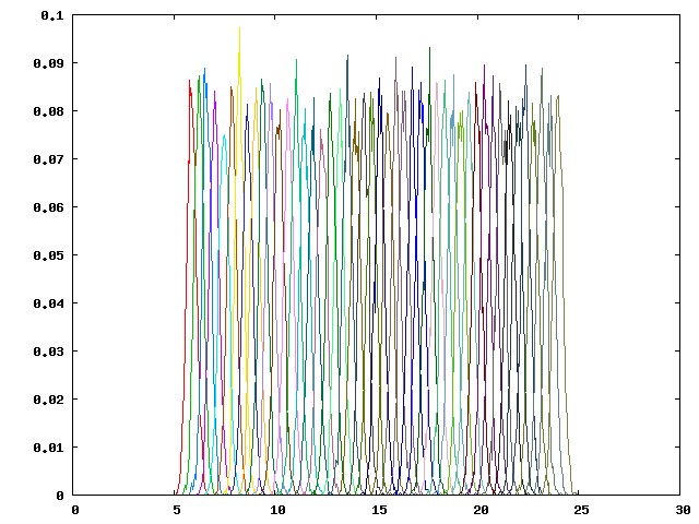
This histogram consists of values in the first column of the hist.dat files from 46 pulling windows (p00-p45), which are the distances between the dummy atom P1 and the guest atom G1. The partial overlapping of the neighboring umbrella sampling windows, as shown above, reflects an adequate sampling along the regions along the potential of mean force (PMF). When there is a large energy barrier along the pulling coordinate, you may observe wide gaps between adjacent umbrella sampling windows, which indicates that the pulling coordinate is poorly sampled. An example of a poorly sampled PMF (from another host-guest system) is provided below:
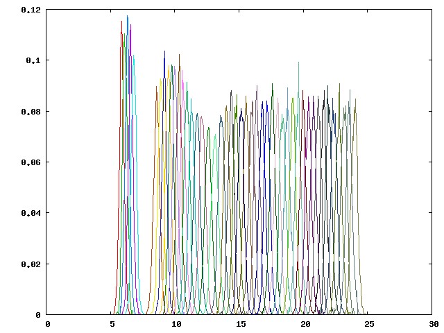
The wide gap between windows p04 (cyan line near the gap) and p05 (brown line near the gap) indicates that the distance restraint between P1 and G1 is not strong enough to hold the guest at the predefined position. Therefore, the actual pulled distance of the guest deviates significantly from the target distance. Such sampling problems can be resolved by adding additional conformational restraints to the host:
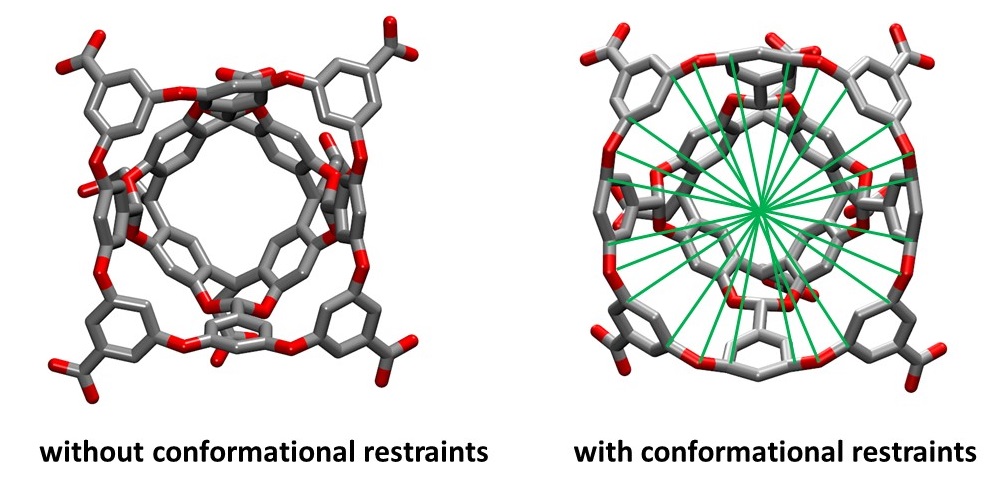
The green lines represent the distance restraints imposed on pairs of atoms across the entrance of the host cavity. These restraints are called "jacks" in the APR input file and can be turned on by defining a set of atoms using the "jacks_list" entry. Simply increasing the restraint force constant for problematic windows and rerunning usually cannot solve the problem because that will very likely lead to enormously large force constants and thus large uncertainties.
If the histogram looks fine, you can now issue the command
(in ./APR)
python apr.py analysis -i apr.in
to compute the work required to attach the restraints to the guest molecule (Wattach), the work required to pull the guest out of the binding pocket (Wpull), and for those cases where the conformational restraints are applied to the host, the work of releasing all attached restraints (Wrelease-conf). This script also computes the work of releasing the guest to standard concentration (Wrelease-std). The thermodynamic integration (TI) approach was used to compute the work from the mean force in each window.
Your output of the TI analysis should look similar to this:
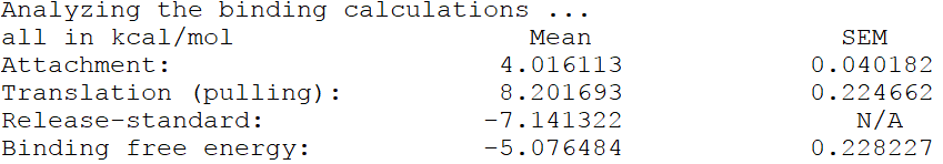
The accumulative work and uncertainties (SEM) from each phrase are provided in TI_attachment.dat and TI_translation.dat. The binding free energy at 1 M standard concentration is computed using the following equation:
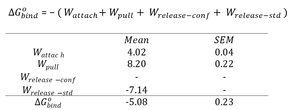
The term of Wrelease-conf is absent in the output because conformational restraints are not imposed. The uncertainty of the binding free energy is computed by adding the errors of all components in quadrature. You may get results that are not exactly the same as those shown here, but they should agree within the range of uncertainties. You might also get slightly different numbers each time running the analysis module, which is normal due to the built-in bootstrapping procedure in the APR workflow. For comparison, the experimental binding affinity of OA – 4-cyanobenzoic acid complex is - 4.25 ± 0.01 kcal/mol measured by NMR, and - 4.73 ± 0.01 kcal/mol measured by ITC. (See Sullivan et al., Yin et al., Mobley and Gilson).
We will introduce how to compute the binding enthalpies in the next section.