5.7 Calculating ion distributions around DNA Using 3D-RISM

by Tiannah York Van Elslande, Felipe Silva Carvalho, Tyler Luchko

Based on work in¹

Giambaşu, G. M.; Luchko, T.; Herschlag, D.; York, D. M.; Case, D. A. Ion Counting from Explicit-Solvent Simulations and 3D-RISM. Biophysical Journal 2014, 106 (4), 883–894. https://doi.org/10.1016/j.bpj.2014.01.021.

Learning Outcomes

By the end of this tutorial, you should be able to

• explain the difference between 1D- and 3D-RISM,
• set up and run 1D-RISM to compute the properties of a bulk liquid,
• visualize the radial distribution functions produced by 1D-RISM,
• use the output from 1D-RISM to calculate a solvent distribution around a solute using 3D-RISM,
• interpret the thermodynamic output from 3D-RISM, and
• visualize the 3D solvent density distribution around the solute molecule.

Introduction: What is 3D-RISM?

The 3D reference interaction site model (3D-RISM)^2–4 of molecular solvation is an implicit solvent model based on the Ornstein-Zernike integral equation that calculates the equilibrium density distribution of an explicit solvent model around a solute on a 3D grid. This information can be used to compute equilibrium thermodynamics, such as the solvation free energy, and the associated thermodynamic density distributions around the solute⁵. 3D-RISM is typically used for trajectory analysis, but it can also be used as an implicit solvent model for molecular dynamics simulations or energy minimization. However, while 3D-RISM is much faster than explicit solvent for calculating solvation thermodynamics on static structures, it is very computational expensive for calculating dynamics.

3D-RISM calculations require two steps.

1. 1D-RISM calculates the bulk properties of the liquid model at a specific temperature and density. The liquid model consists of explicit solvent models of one or more molecular species; e.g., water, sodium and chloride. This information is stored in an xvv file and may be reused with an solute.
2. 3D-RISM calculates the density distribution of this solvent around the solute molecule(s). The solute is modeled with standard force-fields, using standard Amber topology and coordinate files.

The ‘1D’ in ‘1D-RISM’ refers to the fact that only the separation distance between solvent sites is considered, while 3D-RISM includes the orientation of the solute molecule and uses 3D grids. This is the original RISM theory⁶.

Note that RISM theory does not deal with individual atoms or molecules. Rather, it treats the liquid as a collections of molecular species, such as water, methanol, or sodium, which contain sites that have radially symmetric potentials. E.g., in calculation you may specify the density of a water model species and the water model may have oxygen and hydrogen sites. In this example, because the two hydrogen atoms have the same potential, RISM can treat them as a single site with double the density of oxygen – the full geometry of the three atom locations is still used, even though we have only one hydrogen site.

Running 1D-RISM

Prepare Solvent by running a 1D-RISM Script

In order to run 3D-RISM calculations, one first needs to acquire the 1D susceptibility function \(\chi^\text{vv}(r)\) (check chapter 7 of Amber 2023 Reference Manual for further details). This information is obtained by running 1D-RISM calculation on the solvent and it is stored in a xvv file.

1. Create a Directory for 1D-RISM Calculations

In your current working directory, execute the following commands to create some directories for this tutorial:

mkdir rism_dna_ion_tutorial
cd rism_dna_ion_tutorial
mkdir 1-solvent
cd 1-solvent

Now the input file for the 1D-RISM calculation can be created.

2. 1D-RISM inp file

The rism1d program requires an input file with runtime parameters, which must have a .inp suffix. The following is the first half of the input file:

&PARAMETERS
OUTLIST='gx', THEORY='DRISM', CLOSURE='PSE4',
!grid
NR=16384, DR=0.025,
!MDIIS
MDIIS_NVEC=20, MDIIS_DEL=0.3, TOLERANCE=1.e-12,
!iter
KSAVE=-1, maxstep=10000,
!bulk solvent properties
TEMPERATURE=298.15, DIEPS=78.44
NSP=3
/

The parameter names are not case sensitive. The Amber manual has many additional parameters that can be utilized. Any parameters not explicitly given in the inp file will use default values listed in the manual.

Let’s take a closer look at the parameter keywords used above.

OUTLIST

List of output files to create, with one character for each file. In the example here x is the site-site susceptibility in reciprocal space (xvv file), and g is the solvent site-site pair distribution function in real space (gvv file), also known as the ‘radial distribution function’. These are the most commonly used output files, but many others output files can be requested. See the Amber Manual for details.

THEORY

Type of RISM theory to use – one of XRISM or DRISM. DRISM uses the dielectrically consistent RISM equation⁷, which requires DIEPS to define the dielectric constant of the liquid. XRISM uses extended RISM theory⁸, which gives the dielectric constant of an ideal gas. Most users will want DRISM, especially for ionic solutions. In this case, DIEPS should be the dielectric constant of the liquid without ions.

CLOSURE

Type of closure approximation to use. To solve the RISM equation an additional equation, called the ‘closure equation’ is required. The KH (Kovalenko-Hirata) equation⁹ is a good starting point for most systems. For ionic systems, the partial series expansion of order-\(n\) (PSEn) produces better results. PSE1 is equivalent to KH. This example uses PSE4. While it works well in this case, it is sometimes necessary to solve with a lower order closure and then repeat the calculation, which will start from the .sav file, with the next higher order closer. E.g., solving with PSE1, then PSE2, PSE3, and PSE4. The Amber manual has additional tips on how to proceed if the system has convergence issues.

NR

The total grid points.

DR

Grid spacing in real space measured in Ångstroms.

MDIIS_NVEC

Number of previous solutions (vectors) the iterative solver should use with the modified direct inversion of the iterative subspace (MDIIS) method. MDIIS is a non-linear solver used for RISM.¹⁰ 20 previous solutions is usually a good choice for 1D-RISM, though one can increase this value up to 40 if difficulties with convergence arises.

MDIIS_DEL

Step size used in MDIIS. A smaller step size may help with convergence problems but it will slow down the convergence rate.

TOLERANCE

Target root-mean-squared residual tolerance for the self-consistent solution.

KSAVE

Number of iteration between saving intermediate solutions. If KSAVE is less than or equal to zero, a restart file is only written after convergence.

MAXSTEP

Maximum number of iterations to be used in order to converge the system.

TEMPERATURE

Temperature of our system in Kelvin.

DIEPS

Dielectric constant of the bulk solvent. This is a required parameter for DRISM.

NSP

Number of solvent species (i.e., types of molecules) in the solution. This number must be consistent with the number of species in the name list under &SPECIES. NSP=3 indicates that three &SPECIES namelists follow. This is a required parameter.

The second part of the input gives details of the components:

&SPECIES
!cSPCE water
units = 'M' !unit in mol/L
DENSITY = 55.5D0,
!if you have the file in the .inp directory
MODEL = "cSPCE.mdl"
!if loading from amber directory
!MODEL="$AMBERHOME/dat/rism1d/mdl/cSPCE.mdl"
/
&SPECIES
!Sodium
units = 'M'
DENSITY = 0.1D0,
!if you have the file in the .inp directory
MODEL = "Na+.mdl"
!if loading from amber directory
!MODEL="$AMBERHOME/dat/rism1d/mdl/jc_SPCE/Na+.mdl"
/
&SPECIES
!Chloride
units = 'M'
DENSITY = 0.1d0,
!if you have the file in the .inp directory
MODEL = "Cl-.mdl"
!if loading from amber directory
!MODEL = "$AMBERHOME/dat/rism1d/mdl/jc_SPCE/Cl-.mdl"
/

Each &SPECIES namelist must provide DENSITY and MODEL parameters. UNITS for the

DENSITY

Density or concentration of this molecular species. The solution in this example is comprised of water molecules and Na⁺ and Cl^- ions at a concentration of 0.1 M.

UNITS

Units that the DENSITY is expressed in. The default is M (actually concentration in molar units). Alternative units are mM (millimolar), 1/A^3 (number per ų), g/cm^3 (g/cm³) or kg/m^3 (kg/m³).

MODEL

Path and name of the mdl file. The path can be relative or absolute. mdl files contain the parameters of the explicit solvent model for the species.

Either download the Cl-.mdl, Na+.mdl and cSPCE.mdl files or copy them to your 1-solvent directory from your Amber installation:

cp $AMBERHOME/dat/rism1d/mdl/jc_SPCE/Na+.mdl Na+.mdl
cp $AMBERHOME/dat/rism1d/mdl/jc_SPCE/Cl-.mdl Cl-.mdl
cp $AMBERHOME/dat/rism1d/mdl/cSPCE.mdl cSPCE.mdl

cSPCE_NaCl.inp is the complete input file for rism1d.

3. Run 1D-RISM

Next, run rism1d:

rism1d cSPCE_NaCl > cSPCE_NaCl.out

rism1d always adds the .inp suffix to cSPCE_NaCl to find cSPCE_NaCl.

The command will produce four files: cSPCE_NaCl.out (from the file redirect), cSPCE_NaCl.xvv (from x in outlist), cSPCE_NaCl.sav (from ksave=-1, cSPCE_NaCl.gvv (from g in outlist), and cSPCE_NaCl.gvv_dT (from g in outlist with the default entropicdecomp=1).

Trouble-shooting and Overcoming Common error

Input file errors

The inp file uses the Fortran namelist format. Deviating from this format or misspelling a keyword will causes errors. Common mistakes include

• including extra lines that are not part of the namelist (including blank lines),
• spaces at the beginning of the line for the first (&) and and last (/) lines of the namelist, and
• no newline after the last namelist.

Deprecated keywords

Some keywords from older versions of rism1d have been deprecated in favor of more descriptive ones. Using deprecated keywords will produce a warning, not an error, but they may be removed in future versions of rism1d, so it is best to avoid them. Check the latest Amber manual to see if keywords have been changed.

Failure to converge (taking too long while running rism1d)

rism1d calculations should not take longer than a minute to run. You can check your progress in the out file. See the ‘Solution Convergence’ section of the manual for suggests if your calculation is not converging.

No .xvv file:

If x was included in outlist, but no xvv file was produced, check the out file for error messages.

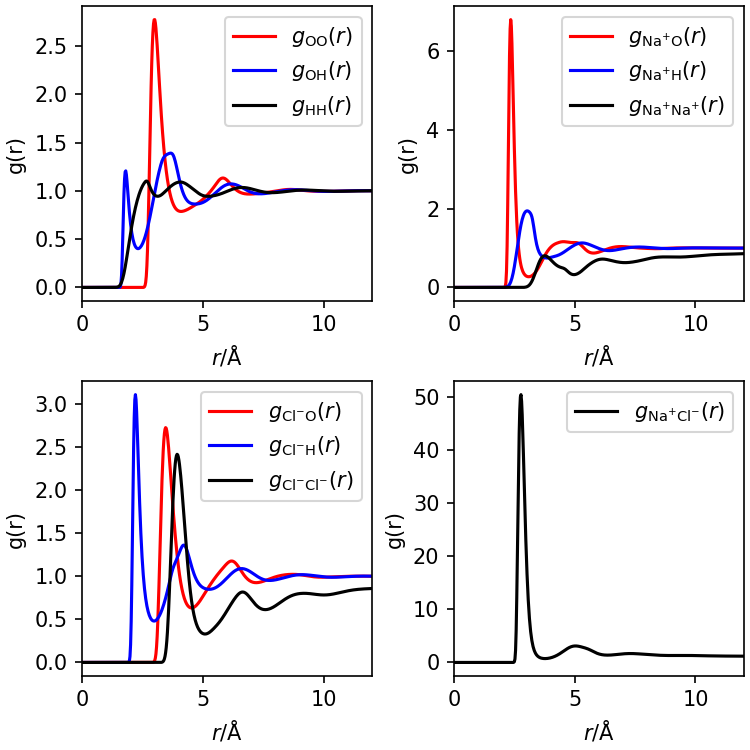
Visualizing the radial distribution functions

Using g in outlist caused rism1d to produce a gvv file, which contains the date for the radial distribution function, \(g(r)\), also called the ‘pair distribution function’. Along with the direct correlation function, \(c(r)\) (cvv file, c in the outlist), the radial distribution function is the primary output of 1D-RISM and is used to calculate all of the thermodynamic properties of the liquid.

The radial distribution tells us the mass/number density of one solvent site around another at a separation \(r\), relative to the bulk. From this we can determine the structure of the liquid. It doesn’t matter which of the pair of sites is at \(r=0\). E.g., \(g_\mathrm{OH}(r)\) is the relative density of H around O and is equal to \(g_\mathrm{HO}\), the relative density of O around H. Since we have four solvent sites in our example (the two hydrogens in water are identical and can be treated as one site), there are 10 pairs of sites and 10 radial distribution functions. You can produce the figure below with this Python script: plotgvv.py. Download it to the same folder containing the gvv file.

3D-RISM

In our example, we will run 3D-RISM on a 24 base-pair strand of DNA, using the xvv we just produced from rism1d.

Add Input Files

To organize our output, create a new directory for our files:

cd ..
mkdir 2-24L
cd 2-24L

The rism3d.snglpnt program we will be using requires pdb, rst7 or nc, and parm7 of the solute. While the calculation is done on the rst7 restart file or nc trajectory file, only one of which should be provided, the pdb file is required. If necessary, you can always generate a pdb file from the parm7 and rst7/nc files with cpptraj; e.g.,

cpptraj -p 24L.parm7 -y 24L.rst7 -x 24L.pdb

We have provided all of the solute input files for this example, which you should download and place in your 2-24L directory: 24L.pdb, 24L.rst7 and 24L.parm7.

You can also use ‘ambpdb’ to generate a pdb file:

ambpdb -p 24L.parm7 -c 24L.rst7 > 24L.pdb

The only other input file we need is the .xvv file we created in the previous section. All parameters are provided as command-line arguments.

Run rism3d.snglpnt

You can run the calculation on a single CPU-core with the command

rism3d.snglpnt --pdb 24L.pdb --prmtop 24L.parm7 --rst 24L.rst7
    --xvv ../1-solvent/cSPCE_NaCl.xvv \
    --closure kh,pse2,pse3 --buffer 48 --grdspc 0.5,0.5,0.5 \
    --verbose 2 --progress --guv g  \
    > 24L.out
    

Depending on your computer, this should take about 1 hour and 30 minutes to complete (4600 s). Alternatively, you can run the calculation in parallel using mpiexec and the rism3d.snglpnt.MPI executable. (Depending on your software and hardware environment, you may need to use a different command than mpiexec and adjust the number of cores from 16 to the number you desire.)

mpiexec -n 16 rism3d.snglpnt.MPI --pdb 24L.pdb --prmtop 24L.parm7 --rst 24L.rst7
    --xvv ../1-solvent/cSPCE_NaCl.xvv \
    --closure kh,pse2,pse3 --buffer 48 --grdspc 0.5,0.5,0.5 \
    --verbose 2 --progress --guv g  \
    > 24L.out

This example with 16 cores should run about 11 times faster.

Parameters

Many parameters can be set on the command line that affect the solution and output of rism3d.snglpnt. Only six parameters are set here. Additional information about the parameter keywords used in rism3d can be found in the Amber manual.

closure

Closure approximation to use. In this example, we used a closure-chain, which can help with higher-order PSEn closures. Our goal is to solve 3D-RISm with the PSE3 closure. First, a high tolerance solution is computed with the kh closure, which is used as an initial guess for a high tolerance solution with the pse2 closure, which is used as an initial guess for a low tolerance solution with the pse3 closure.

buffer

Minimum distance in Å between the solute and the edge of the solvation box. Though this is a non-periodic solution, a larger buffer reduces artifacts but increases computation time.

grdspc

Spacing between grid points in Å. Generally, 0.5 Å is the largest grid spacing that should be used. A smaller grid spacing will increase both the size of output files and the computation time required.

verbose

Level of verbosity when writing additional information to the out file. Level 2 is the highest.

progress

Output the residual for each iteration. Requires --verbose 2.

guv

Output a 3D pair distribution grid for each solvent site of each frame of input. The argument is used as the prefix for the filenames. The format is PREFIX.SITE_NAME.FRAME_NUMBER.FORMAT_SUFFIX.

Output Files

In our directory, we should now see the following files:

24L.out      g.Na+.1.mrc  g.O.1.mrc 24L.rst7
g.Cl-.1.mrc  g.H1.1.mrc   24L.pdb   24L.parm7

Please note: If you are using a version of AMBER that is older than AMBER 22, your output files will be DX files by default. These files are larger and text based, but the visualization process is the same.

You can also download copies of the output here: 24L.out, cSPCE_NaCl.gvv.Na+.1.mrc, cSPCE_NaCl.gvv.Cl-.1.mrc, cSPCE_NaCl.gvv.O.1.mrc and cSPCE_NaCl.gvv.H1.1.mrc.

g.*.1.mrc

Binary formatted volumetric data file of the pair distribution function data for each solvent site around the solute. For each file, the * is the site name, and “1” refers to the frame number. For trajectories, a set of files is created for each frame. These files can be used to visualize the solvent density distribution.

24L.out

Output file containing thermodynamic data and information about the iteration procedure.

Thermodynamic data in the out file

Thermodynamic data calculated by rism3d.snglpnt is output in the out file as a table. The contents of the table varies depending on the type of calculation done. However, a description of what is included the current calculation is printed after the mm_options are listed. In our example, this description looks like

|solutePotentialEnergy        [kcal/mol] Total             LJ         Coulomb              ...          3D-RISM
|rism_excessChemicalPotential [kcal/mol] Total   ExcChemPot_O   ExcChemPot_H1   ExcChemPot_Na+   ExcChemPot_Cl-
|rism_solventPotentialEnergy  [kcal/mol] Total UV_potential_O UV_potential_H1 UV_potential_Na+ UV_potential_Cl-
|rism_partialMolarVolume      [A^3]        PMV
|rism_totalParticlesBox       [#]                  TotalNum_O     TotalNum_H1     TotalNum_Na+     TotalNum_Cl-
|rism_totalChargeBox          [e]        Total     TotalChg_O     TotalChg_H1     TotalChg_Na+     TotalChg_Cl-
|rism_excessParticlesBox      [#]                     ExNum_O        ExNum_H1        ExNum_Na+        ExNum_Cl-
|rism_excessChargeBox         [e]        Total        ExChg_O        ExChg_H1        ExChg_Na+        ExChg_Cl-
|rism_excessParticles         [#]                     ExNum_O        ExNum_H1        ExNum_Na+        ExNum_Cl-
|rism_excessCharge            [e]        Total        ExChg_O        ExChg_H1        ExChg_Na+        ExChg_Cl-
|rism_KirkwoodBuff            [A^3]                      KB_O           KB_H1           KB_Na+           KB_Cl-
|rism_DCFintegral             [A^3]                    DCFI_O         DCFI_H1         DCFI_Na+         DCFI_Cl-

The first column describes the thermodynamic quantity, the second provides the units, the third gives the total (if applicable) and the remaining columns (if applicable) give the components.

After each frame is processed, a table is printed with the calculated values. For these tables, there is no leading | at the start of the line.

A more detailed description is given below.

solutePotentialEnergy

[kcal/mol] Total potential energy of the solute and components of the potential energy terms. “...” represents additional columns not shown here. Note that the 3D-RISM term is always the rism_excessChemicalPotential.

rism_excessChemicalPotential

[kcal/mol] Total excess chemical potential of the solute, which is also the solvation free energy of the solute, and the contributions from each solvent site.

rism_solventPotentialEnergy

[kcal/mol] Total potential energy between solute and solvent, and the contributions from each solvent site.

rism_partialMolarVolume

[ų] Partial molar volume of the solute.

rism_totalParticlesBox

[#] Number of solvent particles in the solvation box for each solvent site.

rism_totalChargeBox

[e] Total charge of the solvent particles in the solvation box and the contributions from each solvent site.

rism_excessParticlesBox

[#] Number of solvent particles for each solvent site in excess of what would be present for the bulk liquid in the same box.

rism_excessParticals

[#] Number of solvent particles for each solvent site in excess of what would be present for the bulk liquid over all space. This is also called the ‘molar preferential interaction parameter’.

rism_excessCharge

[e] Total charge of solvent particles in excess of what would be present for the bulk liquid over all space. If ions are present, this value should be the same magnitude and opposite sign as the net charge of the solute. Contributions of each site are also provided.

rism_KirkwoodBuff

[ų] Kirkwood-Buff integral. This is the integral of \(g(\vec{r})\) over all space for each site. It appears in calculation of many thermodynamic quantities.

rism_DCFintegral

[ų] Integral of the direct correlation function, \(c(\vec{r})\) integrated over all space. It also appears in many thermodynamic calculations.

Visualizing the Outcome with VMD

Density distributions in mrc files from the calculation may be visualized with software, such as VMD.

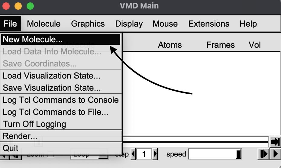
First, open the VMD program. In the VMD main window, click “File” and select “New molecule”.

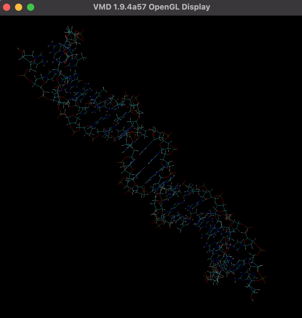
The “Molecule File Browser” will appear and will prompt you to search for a filename. Click the “Browse” button, select the 24L.pdb file from your 2-24L directory. The “Determine File Type” should automatically select “PDB”. Click the “Load” button.

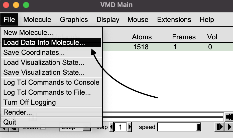
On the “VMD Main” window, make sure the pdb file is selected, then click on the “File” pull-down menu and select “Load Data Into Molecule”. Load each of the mrc files one by one.

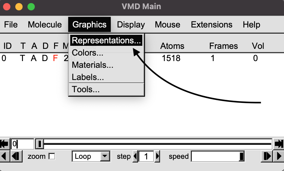
On the VMD Main window, click on the “Graphics” pull-down menu and select “Representations”.

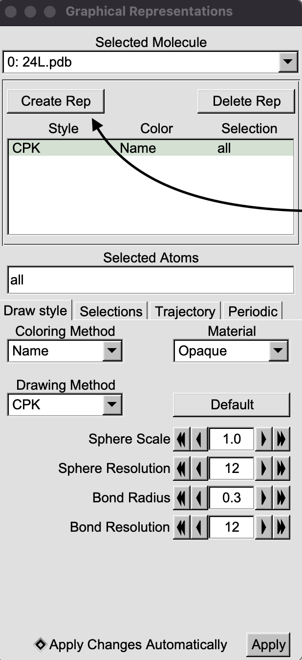
A new Graphical representations window will appear. Click on “Create Rep”.

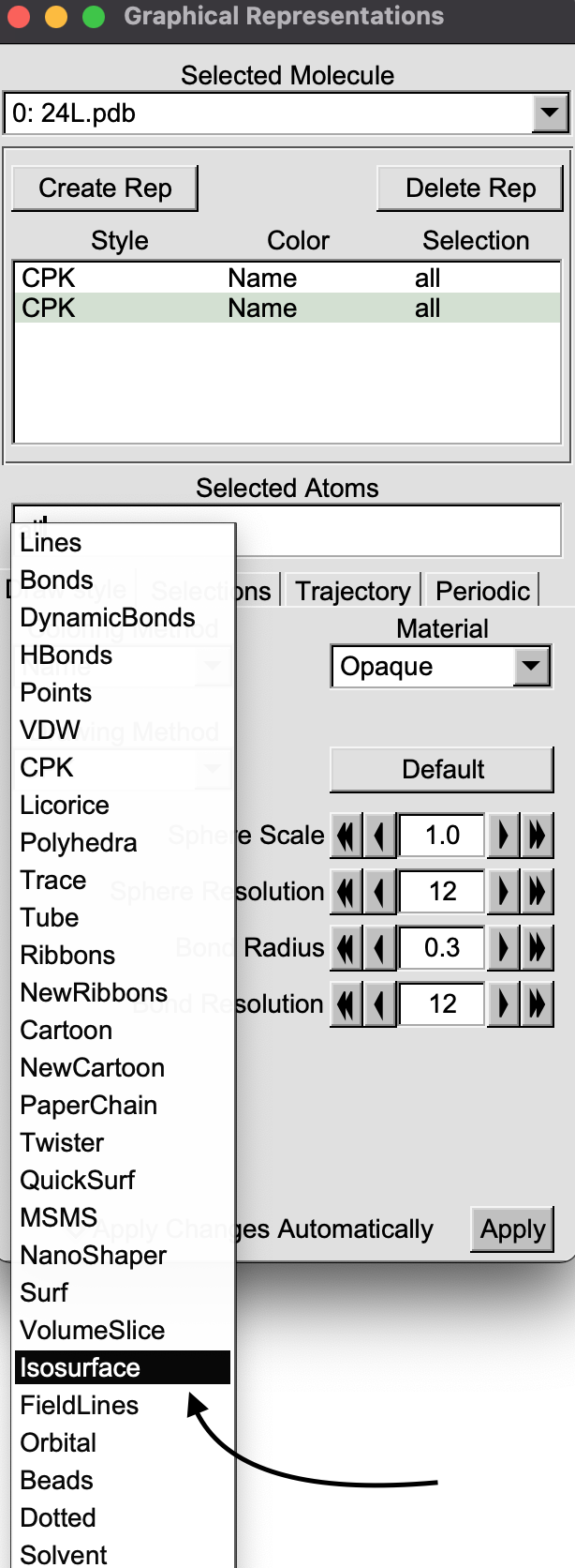
In “Draw Style” tab, click on the “Drawing Method” pull-down menu and select “isosurface”.

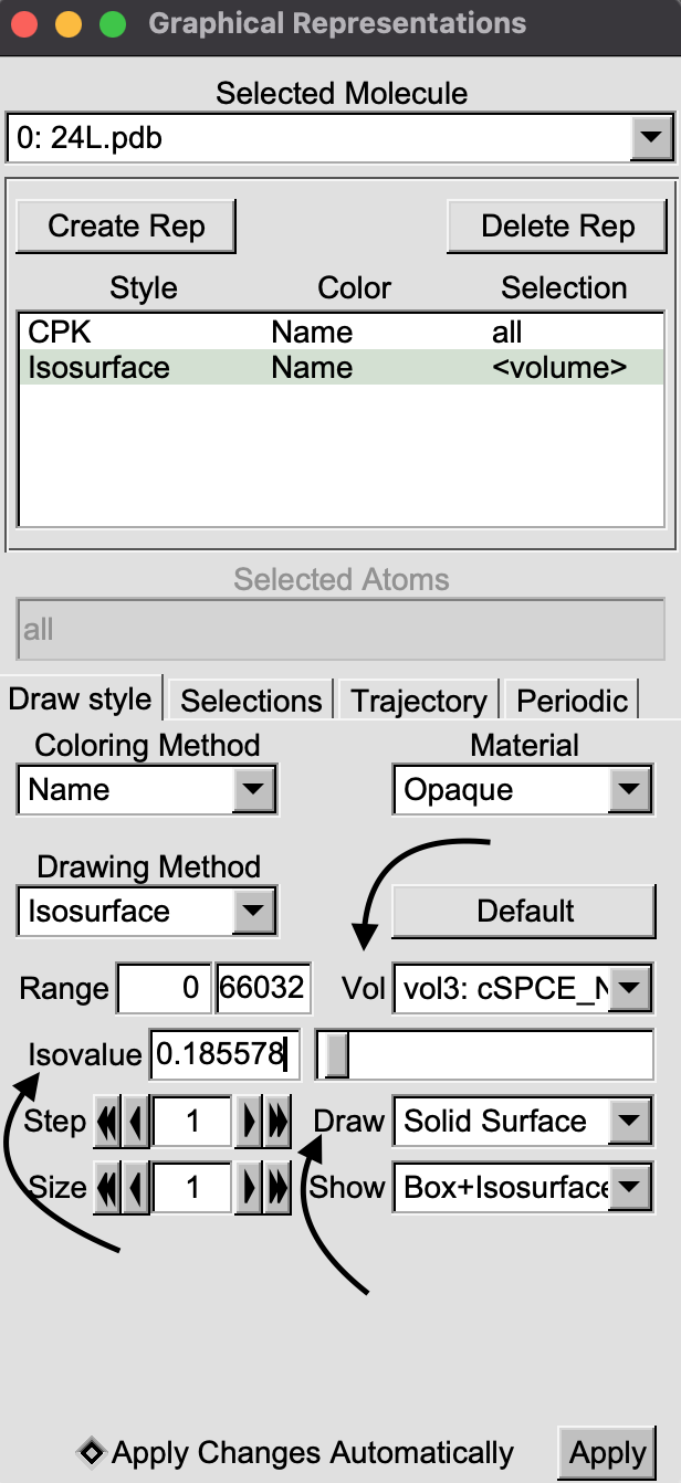
In the VMD display window, a box will appear around the molecule. More options will also appear in the “Graphical Representations” window. On the “Draw” pull-down menu, select “Solid Surface”. Set the “Isovalue” to a value larger than 1 by typing it in or using the slider. This allows you to draw surfaces at different relative densities. You can switch between mrc files by selecting them from the “Vol” pull down menu. By creating multiple representations, you can visualize densities for different sites at the same time.

Every point on the isosurface has the same value of \(g(\vec{r})\), which is the isovalue specified. An isovalue less than 1 (\(g(\vec{r})<1\)) represents a depletion of that species, while a value greater than one (\(g(\vec{r})>1\)) represents an excess. High values of \(g(\vec{r})\), which represent high densities and potential tight binding. Low values of the pair distribution function, that are still larger than 1, indicate diffuse binding. There is no set numerical cutoff between diffuse and tight binding.

Some figures for different Isovalues are presented below:

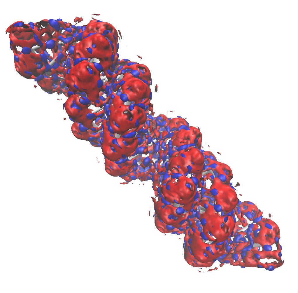
Results for sodium

Setting the isovalue for sodium to 50, we see that sodium accumulates at high density around phosphate backbone of the DNA molecule. Inside the surface, \(g_\mathrm{Na^+}(\vec{r}) > 50\), and outside the surface, \(g_\mathrm{Na^+}(\vec{r}) < 50\).

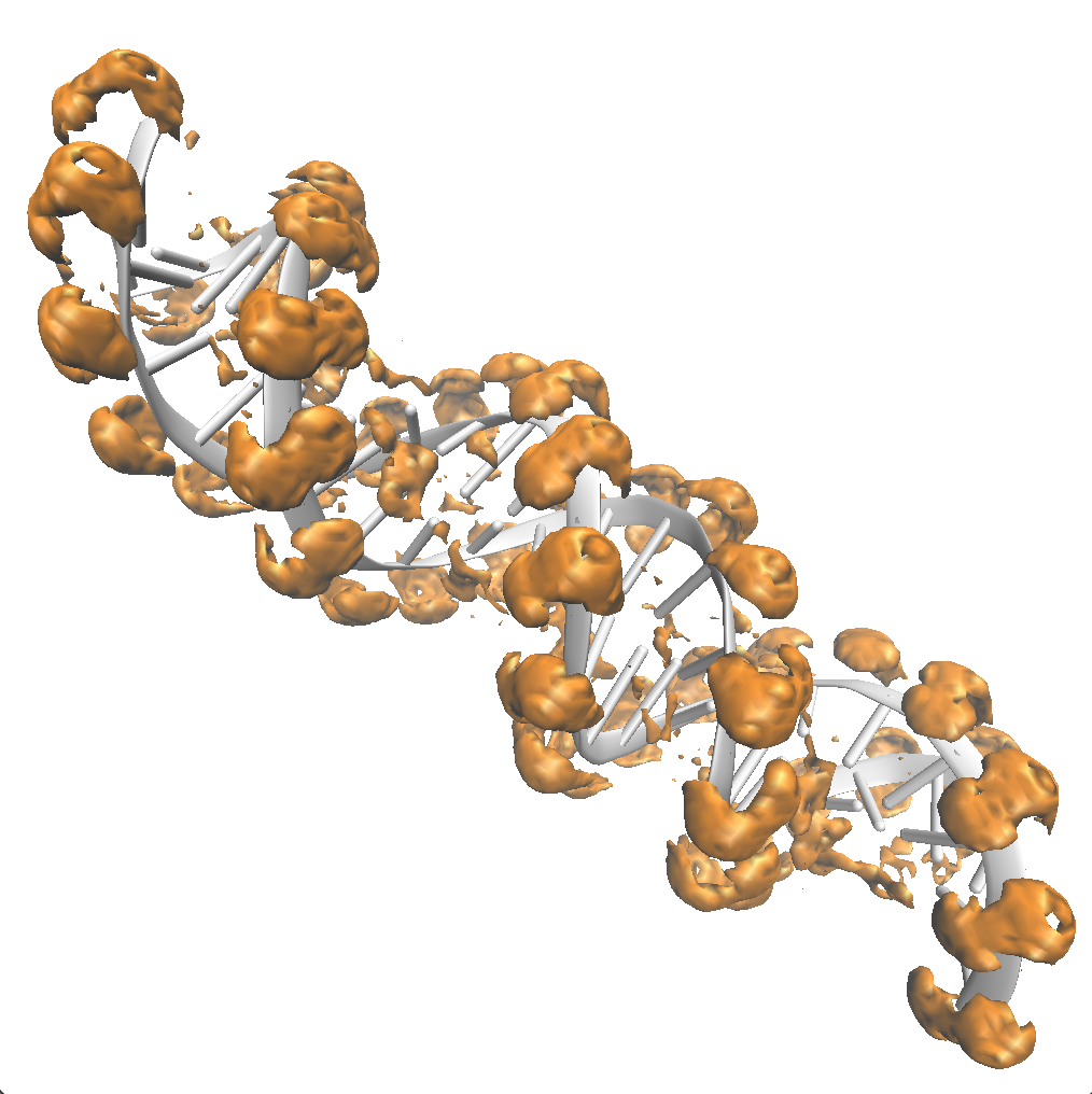
Highlighting the phosphate oxygens with the CPK representation, one can see the cations surrounding these negatively charged atoms.

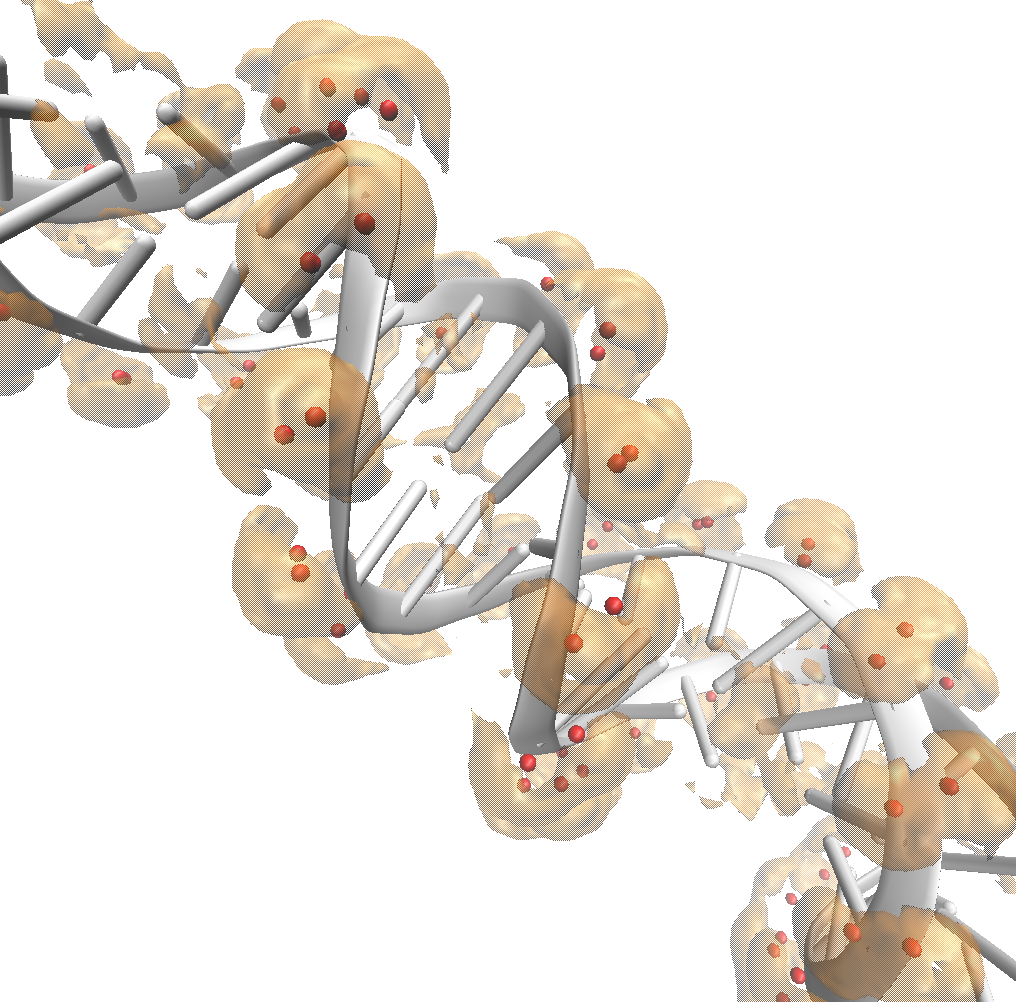
An isovalue of 2 shows diffuse binding between the cations and molecule manifesting as a big bubble. Densities greater than bulk can extends 10s of Ångstroms from the DNA molecule, depending on the concentration of sodium.

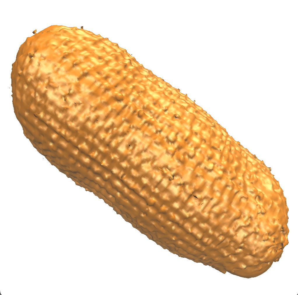
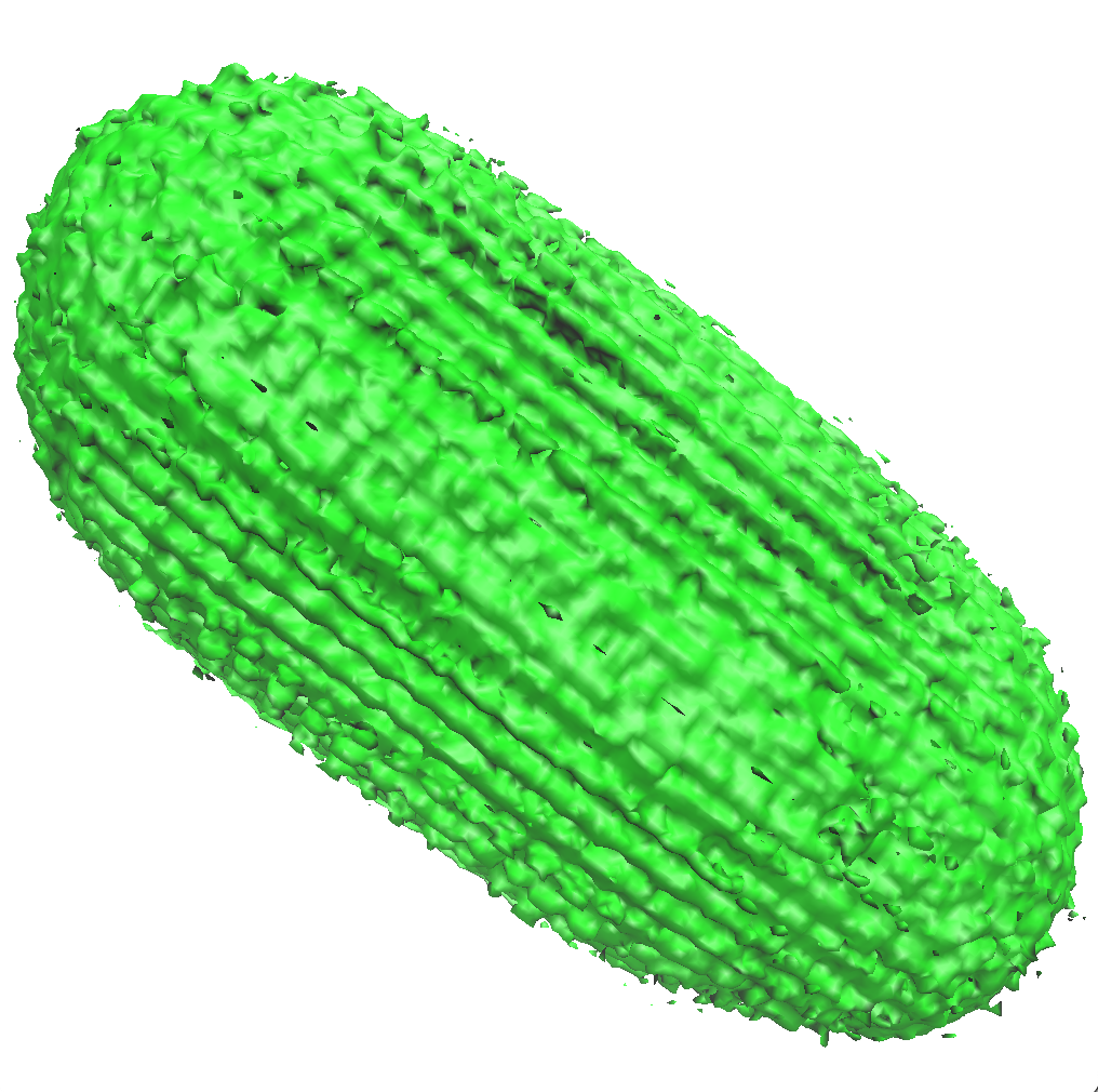
Results for oxygen and hydrogen

Using an isovalue four times the bulk density for both oxygen and hydrogen, we see that the distribution of water is non-uniform close to the surface of the DNA molecule.

Reducing this value to twice the bulk density it is possible to oberve a bigger surface around the DNA and the second solvation shell begins to appear.

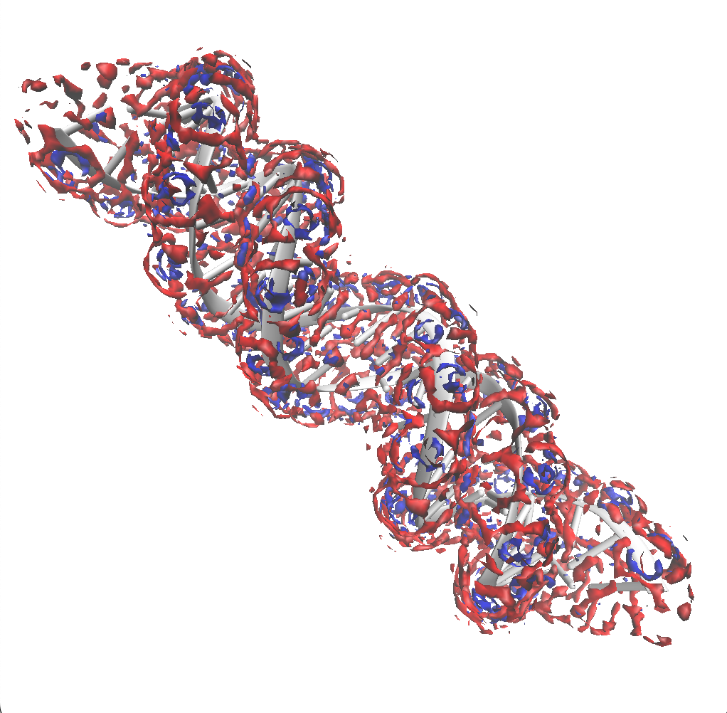
Results for chloride

An isovalue of 2 for chloride shows only a few small regions where this ion binds diffusely with DNA. This occurs at the
end of the DNA, where some positive charge is exposed.

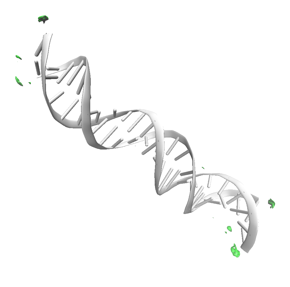
On the other hand, by setting the isovalue to 0.7, one can conclude that the negativelly charged ions are depleted around the molecule. From our view, \(g(\vec{r})<0.7\) inside the surface (near the DNA), except for a few small regions near the termini, as shown above. This should be expected, since the DNA molecule has a net charge about -27 e.

Placing solvent molecules

3D-RISM calculates the density distributions of the solvent and the thermodynamic properties. It does not place solvent atoms around the solute. If you want to place solvent atoms in their most probable locations, see the tutorial on Placing waters and ions using 3D-RISM and MOFT.

References