(Note: These tutorials are meant to provide
illustrative examples of how to use the AMBER software suite to carry out
simulations that can be run on a simple workstation in a reasonable period of
time. They do not necessarily provide the optimal choice of parameters or
methods for the particular application area.)
Copyright Jason Swails and T. Dwight McGee, 2013
Analyzing the Results:
This section describes how to analyze the results obtained from the CpHMD
simulations.
Using cphstats
The various protonation states that are sampled throughout the course of the
CpHMD simulations are written to a cpout file. The program
cphstats can be used to parse the cpout file and for calculating the
predicted pKa values. Use the -h flag to get a full listing
of the available command-line flags for cphstats.
cphstats -i cpin [cpout1 cpout2 cpout3 cpoutN] [-o output] [--population population_ouput]
For example, the command
cphstats -i 4LYT.equil.cpin 0/4LYT.md1.cpout -o pH0_calcpka.dat
--population pH0_populations.dat
will create the following two files for the simulations at pH 0:
pH0_calcpka.dat and pH0_populations.dat
You can use a small shell command to analyze all results at once. For
instance:
for ph in 0 1 2 3 4 5 6 7; do
cphstats -i 4LYT.equil.cpin ${ph}/4LYT.md1.cpout -o
pH${ph}_calcpka.dat --population pH${ph}_populations.dat
done
will create files with the titration statistics for all simulations. We
recommend you generate these files yourself, but a tarball containing these
files are available here: pH_statistics.tar.bz2
| pH0_calcpka.dat |
Solvent pH is 0.000
GL4 7 : Offset 3.387 Pred 3.387 Frac Prot 1.000 Transitions 11
HIP 15 : Offset Inf Pred Inf Frac Prot 1.000 Transitions 0
AS4 18 : Offset 1.992 Pred 1.992 Frac Prot 0.990 Transitions 179
GL4 35 : Offset Inf Pred Inf Frac Prot 1.000 Transitions 0
AS4 48 : Offset 1.635 Pred 1.635 Frac Prot 0.977 Transitions 37
AS4 52 : Offset 1.395 Pred 1.395 Frac Prot 0.961 Transitions 1
AS4 66 : Offset -Inf Pred -Inf Frac Prot 0.000 Transitions 0
AS4 87 : Offset 2.365 Pred 2.365 Frac Prot 0.996 Transitions 13
AS4 101 : Offset 3.979 Pred 3.979 Frac Prot 1.000 Transitions 5
AS4 119 : Offset 1.840 Pred 1.840 Frac Prot 0.986 Transitions 191
Average total molecular protonation: 9.909
|
Offset: is the difference between the predicted pKa and the system pH
Pred: is the predicted pKa
Frac Prot: is the fraction of time the residue spends protonated
Transitions: gives the number of accpeted protonations state transitions
Average total molecular protonation: is the sum of the fractional protonations
cphstats also printed another file with the populations of every
state for every titratable residue, pH0_populations.dat. This file
prints the fraction of snapshots that the system spent in each state for each
residue. For example, His 15 was protonated 100% of the time, whereas Asp 119
was deprotonated 1.42% of the time, syn- protonated ~48% of the time on each
oxygen (this is good since they are rotationally degenerate!), and
anti-protonated ~0.7% of the time.
| pH0_populations.dat |
Residue Number State 0 State 1 State 2 State 3 State 4
-----------------------------------------------------------------------------------
Residue: GL4 7 0.000410 (0) 0.453512 (1) 0.004275 (1) 0.535908 (1) 0.005895 (1)
Residue: HIP 15 1.000000 (2) 0.000000 (1) 0.000000 (1)
Residue: AS4 18 0.010085 (0) 0.486042 (1) 0.004335 (1) 0.495922 (1) 0.003615 (1)
Residue: GL4 35 0.000000 (0) 0.581343 (1) 0.000360 (1) 0.368002 (1) 0.050295 (1)
Residue: AS4 48 0.022640 (0) 0.520073 (1) 0.018440 (1) 0.425152 (1) 0.013695 (1)
Residue: AS4 52 0.038725 (0) 0.517533 (1) 0.113676 (1) 0.280601 (1) 0.049465 (1)
Residue: AS4 66 1.000000 (0) 0.000000 (1) 0.000000 (1) 0.000000 (1) 0.000000 (1)
Residue: AS4 87 0.004295 (0) 0.439747 (1) 0.010535 (1) 0.524678 (1) 0.020745 (1)
Residue: AS4 101 0.000105 (0) 0.504673 (1) 0.013110 (1) 0.478517 (1) 0.003595 (1)
Residue: AS4 119 0.014240 (0) 0.488767 (1) 0.007100 (1) 0.483272 (1) 0.006620 (1)
|
NOTE: The parentheses (*), indicates the number protons present in that state.
The cpout file can be divided into chunks of time using
calcpka. This feature is enabled when a dump_interval, is
specified (using the -t flag on the command-line). The information is
printed to the file pKa_evolution.dat if the -ao flag is not
given.
Calculating the pKas
Here we will look at a couple ways of computing pK
a values using the
output from
calcpka. The predicted pK
as printed in the
calcpka output assumes ideal, Hendersen-Hasselbalch titration behavior
obeying the equation:
pK_a=pH-\log\frac{[A^-]}{[HA]}"
[1]
In proteins, titration behavior for each titratable residue is not always
this straight-forward, and two or more residues may impact each others'
titration curves. Therefore, the Hill equation, shown below, is typically used
to fit titration curves and calculate pKas.
pK_a = pH - n \log \frac {[A^-]} {[HA]}
[2]
The trick now becomes to plot our titration curve—typically plotted as
the deprotonated fraction (which is directly related to [A-]) versus
pH. Knowing that f_d = \frac{[A^-]} {[HA] + [A^-]},
where fd is the fraction deprotonated, we can rearrange
Equation 2 to obtain:
f_d = \frac 1 {1 + 10 ^ {n (pK_a - pH)}}
[3]
Now the trick is to extract the deprotonated fraction from the
calcpka output shown above (which is just 1 − fraction
protonated) for each residue as a function of the pH. The data is shown below,
where the first column is the pH and the subsequent columns are the deprotonated
fraction for each residue.
| titration_curves.dat |
# pH GLU7 HIS15 ASP18 GLU35 ASP48 ASP52 ASP66 ASP87 ASP101 ASP119
0.000 0.000 0.000 0.010 0.000 0.023 0.039 1.000 0.004 0.000 0.014
1.000 0.006 0.000 0.098 0.000 0.276 0.312 1.000 0.015 0.002 0.069
2.000 0.021 0.000 0.342 0.000 0.977 0.387 0.999 0.009 0.014 0.546
3.000 0.186 0.001 0.789 0.000 0.985 0.918 1.000 0.116 0.089 0.598
4.000 0.774 0.004 0.981 0.002 0.998 0.999 1.000 0.633 0.516 0.994
5.000 0.973 0.055 0.999 0.002 1.000 1.000 1.000 0.954 0.933 0.999
6.000 0.999 0.405 0.999 0.037 1.000 1.000 1.000 1.000 0.989 1.000
7.000 0.999 0.826 1.000 0.330 1.000 1.000 1.000 0.999 0.999 1.000
|
In this case, I use gnuplot to fit all of this data to Equation
3 using gnuplot's built-in fitting functionality. This
function needs to be fit using a non-linear, least-squares fitting algorithm
(e.g., the Marquardt-Levenberg algorithm). As a result, you should
choose a reasonable starting guess for the fit (the predicted pKa
printed out by calcpka for the pH with the lowest offset value is a
good starting point). The gnuplot script shown below will fit all of the
titration curves, plot them, and print the calculated pKa and Hill
coefficients. I wrote a gnuplot tutorial
(available here) if you
wish to better understand what each line in the script is doing.
| titration_curves.gpi |
set terminal png font "Helvetica,16" enhanced size 1680,1200
set output "titration_curves.png"
# Define the titration curve Hill equation
f(x) = 1 / (1 + 10**(n*(pka - x)))
# Set up the x- and y-ranges
set xrange[0:7]
set yrange[0:1]
# Turn on grid
set grid linewidth 0
# Turn off the key, we will use labels instead
unset key
# Set up a multiplot
set multiplot layout 3,4
# Fit the first residue
set title 'Glu 7'
pka = 3.5; n = 1.0 # initial guesses
fit f(x) 'titration_curves.dat' using 1:2 via n,pka
set label 1 sprintf("pK_a = %.2f\nn = %.2f", pka, n) at graph 0.05,0.3
plot 'titration_curves.dat' using 1:2 with points pointsize 2, \
f(x) with lines linewidth 2
# Fit the second residue
set title 'His 15'
pka = 6.5; n = 1.0 # initial guesses
fit f(x) 'titration_curves.dat' using 1:3 via n,pka
unset label 1
set label 2 sprintf("pK_a = %.2f\nn = %.2f", pka, n) at graph 0.05,0.3
plot 'titration_curves.dat' using 1:3 with points pointsize 2, \
f(x) with lines linewidth 2
# Fit the third residue
set title 'Asp 18'
pka = 2.5; n = 1.0 # initial guesses
fit f(x) 'titration_curves.dat' using 1:4 via n,pka
unset label 2
set label 3 sprintf("pK_a = %.2f\nn = %.2f", pka, n) at graph 0.5,0.3
plot 'titration_curves.dat' using 1:4 with points pointsize 2, \
f(x) with lines linewidth 2
# Fit the fourth residue
set title 'Glu 35'
pka = 7.5; n = 1.0 # initial guesses
fit f(x) 'titration_curves.dat' using 1:5 via n,pka
unset label 3
set label 4 sprintf("pK_a = %.2f\nn = %.2f", pka, n) at graph 0.05,0.3
plot 'titration_curves.dat' using 1:5 with points pointsize 2, \
f(x) with lines linewidth 2
# Fit the fifth residue
set title 'Asp 48'
pka = 1.5; n = 1.0 # initial guesses
fit f(x) 'titration_curves.dat' using 1:6 via n,pka
unset label 4
set label 5 sprintf("pK_a = %.2f\nn = %.2f", pka, n) at graph 0.5,0.3
plot 'titration_curves.dat' using 1:6 with points pointsize 2, \
f(x) with lines linewidth 2
# Fit the sixth residue
set title 'Asp 52'
pka = 2.5; n = 1.0 # initial guesses
fit f(x) 'titration_curves.dat' using 1:7 via n,pka
unset label 5
set label 6 sprintf("pK_a = %.2f\nn = %.2f", pka, n) at graph 0.5,0.3
plot 'titration_curves.dat' using 1:7 with points pointsize 2, \
f(x) with lines linewidth 2
# Plot the seventh residue (do not fit, since it does not titrate)
set title 'Asp 66'
unset label 6
plot 'titration_curves.dat' using 1:8 with points pointsize 2
# Fit the eight residue
set title 'Asp 87'
pka = 3.5; n = 1.0 # initial guesses
fit f(x) 'titration_curves.dat' using 1:9 via n,pka
set label 8 sprintf("pK_a = %.2f\nn = %.2f", pka, n) at graph 0.05,0.3
plot 'titration_curves.dat' using 1:9 with points pointsize 2, \
f(x) with lines linewidth 2
# Fit the ninth residue
set title 'Asp 101'
pka = 4.0; n = 1.0 # initial guesses
fit f(x) 'titration_curves.dat' using 1:10 via n,pka
unset label 8
set label 9 sprintf("pK_a = %.2f\nn = %.2f", pka, n) at graph 0.05,0.3
plot 'titration_curves.dat' using 1:10 with points pointsize 2, \
f(x) with lines linewidth 2
# Fit the tenth residue
set title 'Asp 119'
pka = 2.5; n = 1.0 # initial guesses
fit f(x) 'titration_curves.dat' using 1:11 via n,pka
unset label 9
set label 10 sprintf("pK_a = %.2f\nn = %.2f", pka, n) at graph 0.5,0.3
plot 'titration_curves.dat' using 1:11 with points pointsize 2, \
f(x) with lines linewidth 2
unset multiplot
|
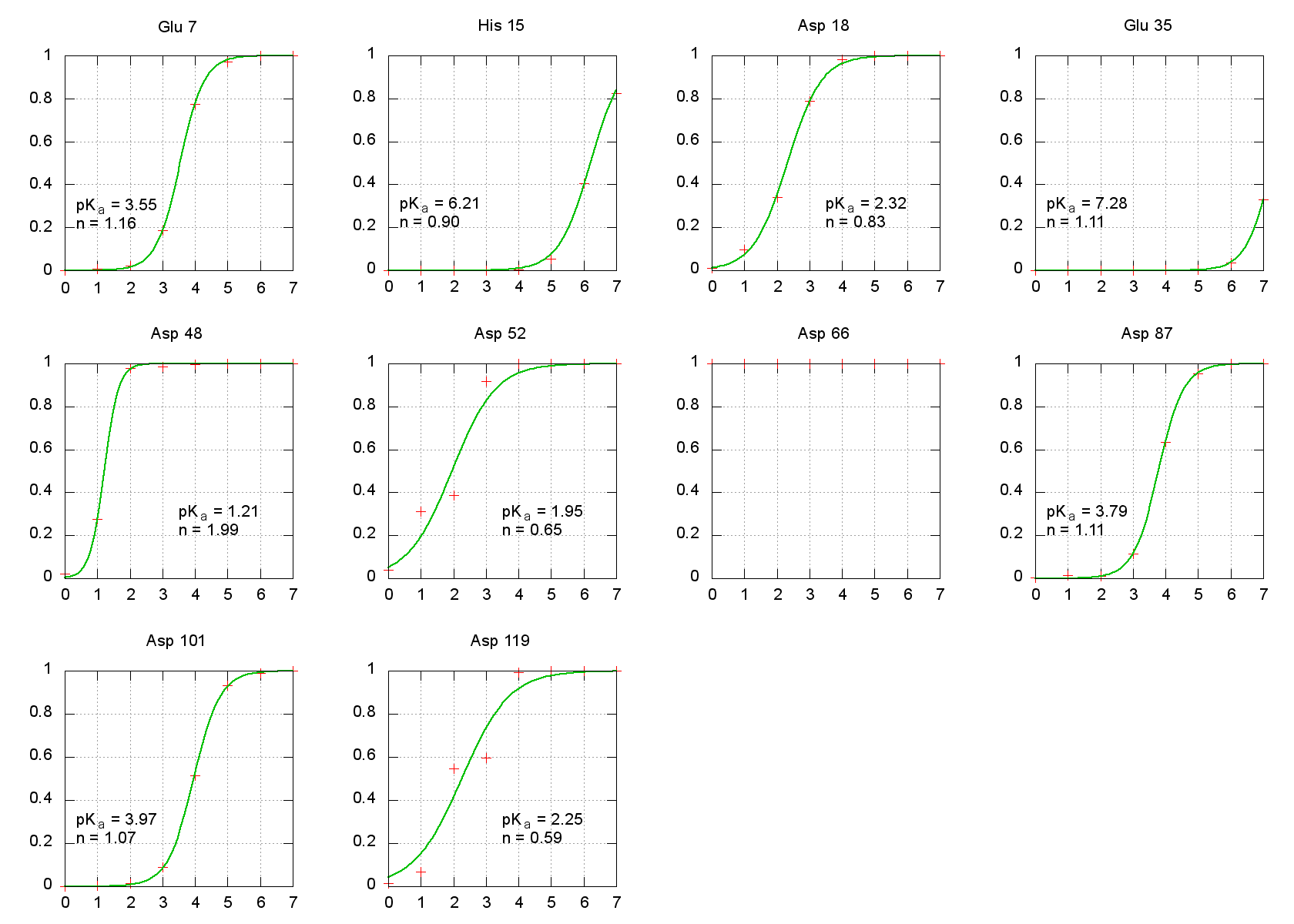
The calculated pKas here show very good qualitative agreement with
experimental measurements for HEWL pKas. Glu 35, whose pKa
has been measured near 6.1, is correctly predicted to have a large shift away
from the model compound pKa of 4.4 for an isolated Glutamate. In each
case, this method correctly predicts the direction of the pKa shift
from the model compound, and even gives quantitatively reasonable results for
most residues as well. Keep in mind, though, that we ran only 1 ns simulations
at each pH, which is most likely insufficient for extensive conformational
sampling. It remains, however, illustrative in demonstrating how to carry out
CpHMD simulations and calculate resulting pKas.
Comparing the Root Mean Squared Deviations of the CpHMD Simulations
Next, we calculate the rmsd of each the CpHMD simulations and histogram the data
using cpptraj.
| cpptraj.rmsd.in |
#calculate the rmsd and histogram the data
trajin 0/4LYT.md1.nc
reference 4LYT.equil.rst7
rmsd rmsph mass reference @CA,C,N,O out pH0.4LYT.rmsd.dat
hist rmsph,*,*,.1,* norm out pH0.4LYT.rmsd.histogram.dat
|
The input shown above is using the trajectory for pH 0 and can be modified to
work with any of the other pH values. The coordinates from
4LYT.equil.rst7 were used as the reference structure and the rmsd of only
the backbone atoms were considered. The hist function in cpptraj was
used to histogram the data. The bin width is set to .1, and the wildcards (*)
tell cpptraj to use the smallest and largest values of the data set to set the
smallest and highest bin, respectively. The last wild-card tells cpptraj to use
the number of bins necessary to go from the data set minimum to the data set
maximum using a step size of 0.1 Angstroms. See the AmberTools manual for more
detailed instructions on using cpptraj.
The data can be generated by executing the following command:
cpptraj 4LYT.parm7 cpptraj.rmsd.in
A tarball containing all of the rmsd and histogram files can be downloaded here:
rmsd_data.tar.bz2
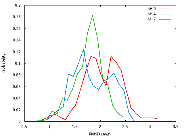
Because our simulations were relatively short and we only have 1000 data
points, the histograms appear pretty noisy. However, we can qualitatively say
that the high pH and low pH simulations were more flexible and explored
conformations farther from the crystal structure. This makes sense, since HEWL
is most active near pH 4, and 4LYT was solved at pH 4.8. [2]
Visualizing the trajectories in VMD
If you do not already know how to use VMD with Amber files, please see
Basic Tutorial 2 for
instructions
The trajectories of the CpHMD simulations can be viewed using VMD. The
program VMD_pH.py (along with
getatms.py) get_creates a tcl script to load into
VMD with your topology and trajectory file. This will script will allow you to
see the different protonation states sampled by the protein during the CpHMD
simulations. VMD_pH.py is inefficient for large trajectories, and was written
quickly with limited knowledge of VMD's scripting environment.
VMD_pH.py should be used as:
VMD_pH.py cpin cpout1 cpout2 cpout3 cpoutN...
where the cpin file is just parsed for which residues are titrating (so it
should typically be the cpin file written by cpinutil.py). The cpout
files must be listed in the same order as the trajectories are loaded into VMD
(the full records in the cpout file are matched to each frame of the
trajectory). For large numbers of snapshots, this script becomes very
inefficient.
Perfoming the command below will create a file named
pHVMDscript.tcl that can be loaded into VMD.
VMD_pH.py 4LYT.equil.cpin 0/4LYT.md1.cpout
This particular script identifies the titratable protons that are "gone" for
each residue in each frame, then moves those hydrogen atoms 99 Angstroms away in
each direction. Therefore, we need to use the Dynamic Bonds
representation in VMD to avoid drawing all of the bonds to the H-atoms we have
moved away from the protein.
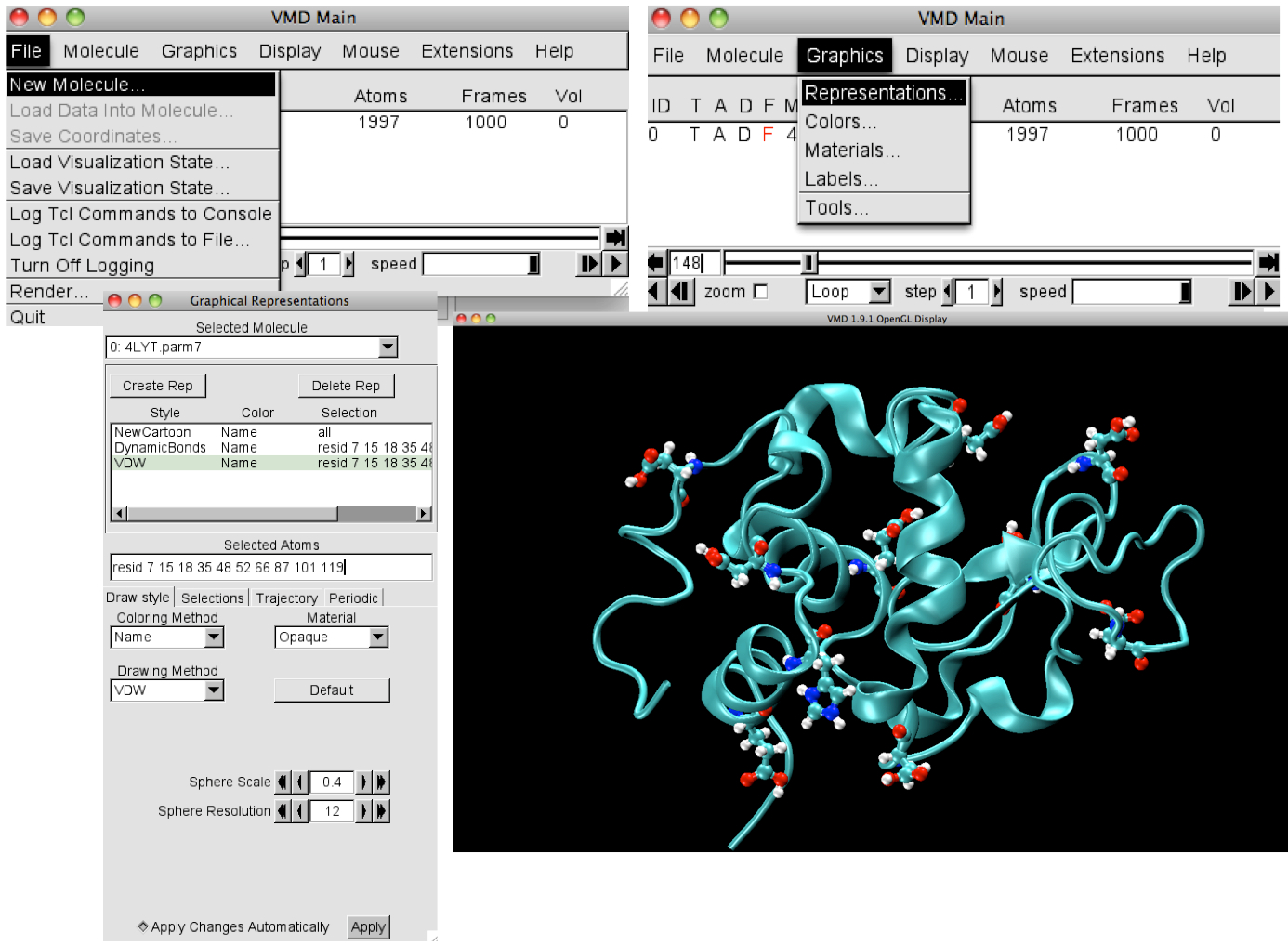
Loading the files in VMD
- Open VMD
- In the console titled VMD Main, click File, followed by
New Molecule
- Load the topology file, 4LYT.parm7, (AMBER 7 Parm) format,
followed by the trajectory file, 0/4LYT.md1.nc, (NetCDF AMBER,MMTK)
format
- In the vmd terminal type source pHVMDscript.tcl
- In the console titled VMD Main click Graphics, followed
by Representations
- Change the drawing method in Graphical Representations console to
New Cartoon
- Click the tab Create Rep and under Selected Atoms type
resid 7 15 18 35 48 52 66 87 101 119
- Change the drawing method to Dynamic Bonds
- Click the tab Create Rep and change the drawing method to
VDW and reduce the Sphere Scale to 0.4
Click here to go back to the Introduction
Click here to go back to Section 3
References
[2] A. C. M. Young, J. C. Dewan, C. Nave, and R. F. Tilton,
"Comparison of radiation-induced decay and structure refinement from X-ray data
collected from lysozyme crystals at low and ambient temperatures", J. Appl.
Cryst., 1993, 26, pp. 309-319
(Note: These tutorials are meant to provide
illustrative examples of how to use the AMBER software suite to carry out
simulations that can be run on a simple workstation in a reasonable period of
time. They do not necessarily provide the optimal choice of parameters or
methods for the particular application area.)
Copyright Jason Swails and T. Dwight McGee, 2013


