


(Note: These tutorials are meant to provide
illustrative examples of how to use the AMBER software suite to carry out
simulations that can be run on a simple workstation in a reasonable period of
time. They do not necessarily provide the optimal choice of parameters or
methods for the particular application area.)
Copyright Ross Walker 2013
Umbrella Sampling Example Calculating the PMF for Alanine Dipeptide Phi/Psi Rotation - SECTION 2
Umbrella Sampling Example
Calculating the PMF for Alanine Dipeptide Phi/Psi Rotation
By Ross Walker & Thomas Steinbrecher
2) Running the Umbrella Sampling Calculations
Now that we have a relaxed starting structure the next part of the calculation is to run MD on the individual umbrella windows. Selecting the number of windows required as well as the size of restraint used is somewhat of a black art. Again we have the problem that the ideal choice requires knowing the solution before we calculate it. The key point to remember when selecting the number of windows is that the end points must overlap, i.e. window 1 must sample some of window 2 etc.. This essentially means that we cannot go wrong by selecting too many windows except that it will require too much computer time. The force constant similarly has to be big enough to ensure that we do in fact sample the subset of phase space that we want to but not too strong that we make our windows too narrow and stop them from overlapping. Normally one can vary the size of the windows and the constraints as a function of position along the pathway. For example if we looked at the separation of two ions when they are very close in, inside the VDW radius we will need very strong restraints and consequently lots of windows. Then as the distance increases we can use weaker and weaker restraints and so have more widely spaced windows.
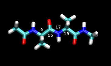
In our example here we will be varying the angle of the C-N bond from 0 to 180 degrees. The image below shows the dihedral we will be varying along with the corresponding atom numbers in the prmtop file (VMD index+1 since VMD numbers from 0)
As a first approximation we shall use umbrella windows spaced 3 degrees apart. This will give us a total of 61 calculations to run. We will use a force constant of 200 KCal/mol rad2 which is larger than the expected barrier height, which should be something in the range of 10 to 30 Kcal thus it should be sufficient to ensure we sample the entire reaction coordinate, but not too large that we will end up with windows that don't overlap. We will check the overlaps once we finish this initial set of calculations and then we can go back and fill in any gaps with extra simulations.
The amount of simulation we do in each window needs to be such we can converge our sampling. Thus if we increase the length with which we run a window the resulting histogram of sampled angles does not change shape. Ideally you would want to run an initial simulation, then calculate the PMF, then throw the last 20% of the data away and calculate the PMF again and see if it changes. If it does not change then your sampling is probably sufficient, if it changes by a marked amount then you likely need to do more sampling.
As a first attempt we will run each window for 150ps where we will throw the first 50ps away as simply being relaxation. Thus for each window from 0 to 180 degrees we will do:
1) Minimization (2000 steps, no shake)
2) Relaxation MD (NPT 50ps, 1fs time step)
3) Data Collection (NPT 100ps, 1fs time step)
One of the issues we need to overcome is the fact that we only have one starting structure (180 degrees). This is a problem since if we start the 0 degree simulation from the 180 degree structure the force of the restraint is just going to pull the structure apart. A more ideal solution would be to run the 180 degree simulation, then use the restart from this as the input for the 177 degree simulation, then use the restart from this for the 174 degree simulation etc. However, such an approach imposes a serial restriction on the calculations so that we can't make use of large scale computer clusters to run the simulation. Thus instead what we will do is manually run the 120 degree simulation, starting from the 180 degree structure (the equilibrium position for alanine-tripeptide that resulted from the earlier relaxation we did) and then manually run the 60 degree simulation started from the final 120 degree structure. This will give us 3 initial structures that we can use as the starting points for the various windows.
The restraints we will be using are AMBER's harmonic restraints that are described in section 4.2 of the AMBER 11 manual. Here is the example input file for the 120 degree minimization, relaxation and data collection case:
| mdin_min.120 | mdin_equi.120 | mdin_prod.120 |
2000 step minimization for 120 deg &cntrl imin = 1, maxcyc=2000, ncyc = 500, ntpr = 100, ntwr = 1000, ntf = 1, ntc = 1, cut = 8.0, ntb = 1, ntp = 0, nmropt = 1, &end &wt type='END', &end DISANG=disang.120 |
50 ps NPT equilibration for 120 deg &cntrl imin = 0, ntx = 1, irest = 0, ntpr = 5000, ntwr = 50000, ntwx = 0, ntf = 2, ntc = 2, cut = 8.0, ntb = 2, nstlim = 50000, dt = 0.001, tempi=0.0, temp0 = 300.0, ntt = 3, gamma_ln = 1.0, ntp = 1, pres0 = 1.0, taup = 5.0, nmropt = 1, ioutfm=1, &end &wt type='END', &end DISANG=disang.120 |
100 ps NPT production for 120 deg &cntrl imin = 0, ntx = 5, irest = 1, ntpr = 10000, ntwr = 0, ntwx = 10000, ntf = 2, ntc = 2, cut = 8.0, ntb = 2, nstlim = 100000, dt = 0.001, temp0 = 300.0, ntt = 3, gamma_ln = 1, ntp = 1, pres0 = 1.0, taup = 5.0, nmropt = 1, ioutfm = 1, &end &wt type='DUMPFREQ', istep1=50, &end &wt type='END', &end DISANG=disang.120 DUMPAVE=dihedral_120.dat |
A couple of things to notice first of all here. I do the minimization without shake. The reason for this is that the sander/pmemd minimizer does not work well with SHAKE, it will minimize the structure but stops quite a way before the minimum. Normally this is not a problem but here, due to the use of the restraints and the less than optimal initial structure I am being more cautious. Then during the two MD runs while I have shake turned on I still use a 1fs time step. This is probably not necessary but again being cautious will not hurt. I also set the pressure relaxation time (taup) to 5ps which is longer than the default of 1ps. This is also to minimize instability problems that might arise. Finally notice that all the files have nmropt=1 set and reference a file called disang.120. This file is what we use to specify the harmonic restraint:
| disang.120 |
| Harmonic restraints for 120
deg &rst iat=9,15,17,19, r1=-60.0, r2=120.0, r3=120.0, r4=300.0, rk2=200.0, rk3=200.0, / |
Here the iat specifies the atom numbers forming the restraint, in this case 9, 15, 17 and 19. Then we specify 4 values r1 to r4 which define the shape of the potential. Essentially between r1 and r2 it will be harmonic with force constant rk2, between r2 and r3 it will be flat and between r3 and r4 it will be harmonic with force constant rk3. In this case we set rk2 = rk3 and r2 = r3 to give us a perfect harmonic potential with a minimum at 120 degrees. It is not required that the potential actually be harmonic, however, the WHAM code we will use in section 3 to generate the PMF assumes that the restraint is a harmonic potential so that is what we will use.
Also note that in the production run we specify a dump frequency of 50 (steps) and an output file of dihedral_120.dat. This means that every 50 steps (50fs) the torsion given by iat will be written to the file dihedral_120.dat.
We can now run these 3 calculations manually to check everything is working correctly (note the 03_equil.rst is the final structure from the first unrestrained relaxation we did, 180 degrees):
mpirun -np 2 $AMBERHOME/bin/pmemd.MPI -O -i mdin_min.120 -o ala_tri_min_120.out -p ala_tri.prmtop -c 03_equil.rst -r ala_tri_min_120.rst
mpirun -np 2 $AMBERHOME/bin/pmemd.MPI -O -i mdin_equi.120 -o ala_tri_equil_120.out -p ala_tri.prmtop -c ala_tri_min_120.rst -r ala_tri_equil_120.rst
mpirun -np 2 $AMBERHOME/bin/pmemd.MPI -O -i mdin_prod.120 -o ala_tri_prod_120.out -p ala_tri.prmtop -c ala_tri_equil_120.rst -r ala_tri_prod_120.rst -x ala_tri_prod_120.nc
Files: ala_tri_min_120.out,
ala_tri_min_120.rst,
ala_tri_equil_120.out,
ala_tri_equil_120.rst,
ala_tri_prod_120.out,
ala_tri_prod_120.rst,
ala_tri_prod_120.nc,
dihedral_120.dat
You should check the calculations to make sure they look okay. The key things to check are that the restraints did not tear things apart going from 180 to 120 degrees and that the restraints appear to be working correctly. In particular we should take a look at the dihedral_120.dat file. We can plot this:
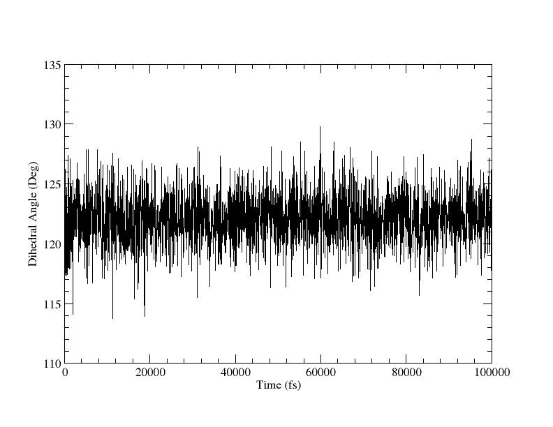
This looks nice although the average is somewhat short of 120 degrees but that is fine since the potential will be biasing it that way, since we are away from the equilibrium position. It could be interpreted as a warning though that our restraint force may not be strong enough. We can also histogram the data so we can check the width:

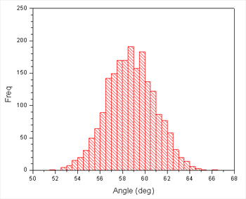
What this tells us is that our restraint force may not be strong enough, since the maximum is around 2.25 degrees from the restraint center. However, we appear to have good sampling and the plot also tells us that 3 degrees is a good separation between windows since the full width half max of the histogram is around 6 degrees. We could probably get away with a slightly wider spacing but it won't do us any harm to be conservative. We also don't need to overly worry about the maximum being offset since the adjacent histograms will provide sufficient overlap.
We can now go on and run the 60 degree simulation manually so we have the three initial structures we will need for the other simulations.
| mdin_min.60 | mdin_equi.60 | mdin_prod.60 |
2000 step minimization for 60 deg &cntrl imin = 1, maxcyc=2000, ncyc = 500, ntpr = 100, ntwr = 1000, ntf = 1, ntc = 1, cut = 8.0, ntb = 1, ntp = 0, nmropt = 1, &end &wt type='END', &end DISANG=disang.60 |
50 ps NPT equilibration for 60 deg &cntrl imin = 0, ntx = 1, irest = 0, ntpr = 5000, ntwr = 50000, ntwx = 0, ntf = 2, ntc = 2, cut = 8.0, ntb = 2, nstlim = 50000, dt = 0.001, tempi=0.0, temp0 = 300, ntt = 3, gamma_ln = 1.0, ntp = 1, pres0 = 1.0, taup = 5.0, nmropt = 1, &end &wt type='END', &end DISANG=disang.60 |
100 ps NPT production for 60 deg &cntrl imin = 0, ntx = 5, irest = 1, ntpr = 10000, ntwr = 0, ntwx = 10000, ntf = 2, ntc = 2, cut = 8.0, ntb = 2, nstlim = 100000, dt = 0.001, temp0 = 300.0, ntt = 3, gamma_ln = 1, ntp = 1, pres0 = 1.0, taup = 5.0, nmropt = 1, ioutfm = 1, &end &wt type='DUMPFREQ', istep1=50, &end &wt type='END', &end DISANG=disang.60 DUMPAVE=dihedral_60.dat |
| disang.60 |
| Harmonic restraints for 60 deg &rst iat=9,15,17,19, r1=-120.0, r2=60.0, r3=60.0, r4=240.0, rk2=200.0, rk3=200.0, / |
Note that for the input structure this time we use the ala_tri_prod_120.rst file produced from the end of the production run of the 120 degree case.
mpirun -np 2 $AMBERHOME/bin/pmemd.MPI -O -i mdin_min.60 -o ala_tri_min_60.out -p ala_tri.prmtop -c ala_tri_prod_120.rst -r ala_tri_min_60.rst
mpirun -np 2 $AMBERHOME/bin/pmemd.MPI -O -i mdin_equi.60 -o ala_tri_equil_60.out -p ala_tri.prmtop -c ala_tri_min_60.rst -r ala_tri_equil_60.rst
mpirun -np 2 $AMBERHOME/bin/pmemd.MPI -O -i mdin_prod.60 -o ala_tri_prod_60.out -p ala_tri.prmtop -c ala_tri_equil_60.rst -r ala_tri_prod_60.rst -x ala_tri_prod_60.nc
Files: ala_tri_min_60.out,
ala_tri_min_60.rst,
ala_tri_equil_60.out,
ala_tri_equil_60.rst,
ala_tri_prod_60.out,
ala_tri_prod_60.rst,
ala_tri_prod_60.nc,
dihedral_60.dat
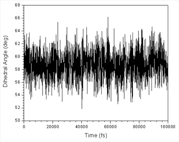
Again you should check that the sampling looks good, check the histogram etc.
Scripting the Runs
Now that we have the necessary starting structures for all the calculations we can write a script to generate all the input files for us, excluding 120 and 60 degrees since we have already run those. The perl scripts below are ones that I wrote to generate all the input files as well as job submission scripts for running on the Teragrid IA64 cluster at the San Diego Supercomputer Center. You will likely need to modify this for your own system. Since each node of the SDSC cluster has 2 processors I will run each job using pmemd.MPI across 2 processors.
The scripts are essentially identical, differing only in the range of angles they calculate. prepare_runs_0-90.perl runs all of the runs from 0 degrees to 90 degrees using the ala_tri_prod_60.rst as the starting structure. prepare_runs_93-147.perl runs 93 degrees to 147 degrees using the ala_tri_prod_120.rst as the starting structure while prepare_runs_150-180.perl runs 150 to 180 degrees using the 03_equil.rst (180 deg) as the starting structure. The example for 0 to 90 degrees is shown below:
#!/usr/bin/perl -w
use Cwd;
$wd=cwd;

print "Preparing input files\n";

$name="ala_tri";
$incr=3;
$force=200.0;

&prepare_input();

exit(0);

sub prepare_input() {

    $dihed=0;
    while ($dihed <= 90) {
      if ($dihed != 60) {
	#skip 60 degrees since we already ran it
	print "Processing dihedral: $dihed\n";
	&write_mdin0();
	&write_mdin1();
	&write_mdin2();
	&write_disang();
	&write_batchfile();
	system("qsub run.pbs.$dihed");
      }
      $dihed += $incr;
    }
}

sub write_mdin0 {
    open MDINFILE,'>', "mdin_min.$dihed";
    print MDINFILE <<EOF;
2000 step minimization for $dihed deg
 &cntrl
  imin = 1,
  maxcyc=2000, ncyc = 500,
  ntpr = 100, ntwr = 1000,
  ntf = 1, ntc = 1, cut = 8.0,
  ntb = 1, ntp = 0,
  nmropt = 1,
 &end
 &wt
  type='END',
 &end
DISANG=disang.$dihed
EOF
    close MDINFILE;
}
sub write_mdin1 {
    open MDINFILE,'>', "mdin_equi.$dihed";
    print MDINFILE <<EOF;
50 ps NPT equilibration for $dihed deg
 &cntrl
  imin = 0, ntx = 1, irest = 0,
  ntpr = 5000, ntwr = 50000, ntwx = 0,
  ntf = 2, ntc = 2, cut = 8.0,
  ntb = 2, nstlim = 50000, dt = 0.001,
  tempi=0.0, temp0 = 300, ntt = 3,
  gamma_ln = 1.0,
  ntp = 1, pres0 = 1.0, taup = 5.0,
  nmropt = 1, ioutfm=1,
 &end
 &wt
  type='END',
 &end
DISANG=disang.$dihed
EOF
    close MDINFILE;
}
sub write_mdin2 {
    open MDINFILE,'>', "mdin_prod.$dihed";
    print MDINFILE <<EOF;
100 ps NPT production for $dihed deg
 &cntrl
  imin = 0, ntx = 5, irest = 1,
  ntpr = 10000, ntwr = 0, ntwx = 10000,
  ntf = 2, ntc = 2, cut = 8.0,
  ntb = 2, nstlim = 100000, dt = 0.001,
  temp0 = 300, ntt = 3,
  gamma_ln = 1.0,
  ntp = 1, pres0 = 1.0, taup = 5.0,
  nmropt = 1, ioutfm=1,
 &end
 &wt
  type='DUMPFREQ', istep1=50,
 &end
 &wt
  type='END',
 &end
DISANG=disang.$dihed
DUMPAVE=dihedral_${dihed}.dat
EOF
    close MDINFILE;
}
sub write_disang {
    $left  = sprintf "%4.1f", $dihed - 180;
    $min   = sprintf "%4.1f", $dihed;
    $right = sprintf "%4.1f", $dihed + 180;
    open DISANG,'>', "disang.$dihed";
    print DISANG <<;
Harmonic restraints for $dihed deg
 &rst
  iat=9,15,17,19,
  r1=$left, r2=$min, r3=$min, r4=$right,
  rk2=${force}, rk3=${force},
 &end
EOF
    close DISANG;
}

sub write_batchfile {
    open BATCHFILE, '>', "run.pbs.$dihed";
    print BATCHFILE <<EOF;
#PBS -l nodes=1:ppn=2
#PBS -l walltime=1:00:00
#PBS -N run_$dihed

cd $wd

mpirun -np 2 -machinefile \$PBS_NODEFILE pmemd.MPI -O \\
-i mdin_min.$dihed -p ${name}.prmtop -c ala_tri_prod_60.rst -r ${name}_min_${dihed}.rst  -o ${name}_min_${dihed}.out
mpirun -np 2 -machinefile \$PBS_NODEFILE pmemd.MPI -O \\
-i mdin_equi.$dihed -p ${name}.prmtop -c ${name}_min_${dihed}.rst  -r ${name}_equil_${dihed}.rst -o ${name}_equil_${dihed}.out
mpirun -np 2 -machinefile \$PBS_NODEFILE pmemd.MPI -O \\
-i mdin_prod.$dihed -p ${name}.prmtop -c ${name}_equil_${dihed}.rst -r ${name}_prod_${dihed}.rst -o ${name}_prod_${dihed}.out -x ${name}_prod_${dihed}.mdcrd
EOF

    print BATCHFILE "\necho \"Execution finished\"\n";
    close BATCHFILE;
}
|
I ran all these calculations on the SDSC Teragrid Cluster. The entire run took about 30 minutes. You are welcome to try running these yourself on your own cluster or you can download a complete set of the outputs (including the 60 and 120 degree runs) here: ala_tri_umbrella_run.tar.gz
Before we move onto the final stage of running WHAM to generate the PMF we should quickly check that all of our windows overlap properly. The easiest way to do this is to plot all of the dihedral_xxx.dat file on the same graph and look for any gaps:
#!/bin/csh
foreach i ( *.dat )
echo $i
cat $i >> all_dihedrals.dat
end
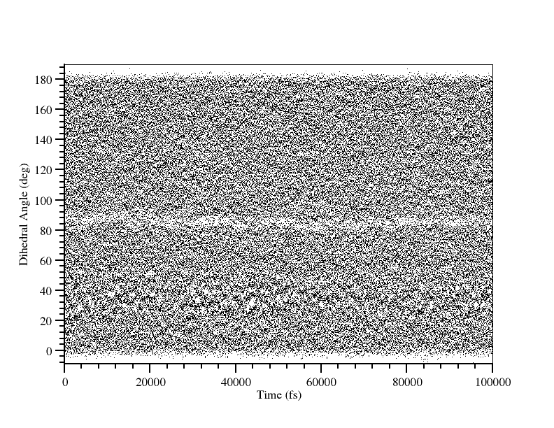
There are no obvious gaps although the data does look a bit sketchy around 81 to 87 degrees. This is most likely the region around the transition state. We can manually plot the histograms for 78, 81, 84, 87 and 90 degrees and check that they all overlap:
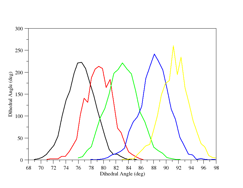
So this shows that there is reduced sampling around 85 degrees but we still have excellent overlap so we should be fine. We can now proceed to section 3 where we will use WHAM to construct our PMF.
(Note: These tutorials are meant to provide
illustrative examples of how to use the AMBER software suite to carry out
simulations that can be run on a simple workstation in a reasonable period of
time. They do not necessarily provide the optimal choice of parameters or
methods for the particular application area.)
Copyright Ross Walker 2013