Umbrella Sampling Example : Introduction

(Note: These tutorials are meant to provide illustrative examples of how to use the AMBER software suite to carry out simulations that can be run on a simple workstation in a reasonable period of time. They do not necessarily provide the optimal choice of parameters or methods for the particular application area.)
Copyright Ross Walker 2013

Umbrella Sampling Example Calculating the PMF for Alanine Dipeptide Phi/Psi Rotation - SECTION 3

Umbrella Sampling Example
Calculating the PMF for Alanine Dipeptide Phi/Psi Rotation

By Ross Walker & Thomas Steinbrecher

3) Constructing the PMF

The final stage of the umbrella sampling is to use the WHAM code of Alan Grossfield to construct our PMF from the dihedral data we collected. The exact workings of WHAM are beyond the scope of this tutorial whose main aim is to show how to perform umbrella sampling in AMBER rather than to provide a course on the theory behind umbrella sampling. For this you should refer to a recent text book on Molecular Dynamics and Statistical Mechanics.

The WHAM code is distributed by Alan Grossfield on his website and can be downloaded there. (There is also a copy available for download from this website wham-dist.tgz)

For this tutorial it is assumed that you have downloaded WHAM, compiled it and put it in /usr/local/bin. Adding it to your PATH means that you should be able to access it by just typing wham and it is assumed from this point forward that that is working correctly.

Now we need to make a wham meta file. This is essentially an input file for wham that tells it the filename of each dihedral file, what the minimum of the harmonic potential was and what the force constant used was.

<filename> <harmonic potential minimum in deg> <force constant in the correct units>

A note on units: Amber uses k(x-x₀)² where k is in kcal/mol/rad² whereas the WHAM program uses 0.5k(x-x₀)² where k is in kcal/mol/deg² hence we have to multiply our original force constants (in this case always 200.0) by 2(pi/180)² = 0.0006092. Thus our force constant in WHAM's units is 0.12184 kcal/mol/deg².

The following script will create our meta.dat file for us:

create_meta.perl

#!/usr/bin/perl -w
use Cwd;
$wd=cwd;

print "Preparing meta file\n";

$name="meta.dat";
$incr=3;
$force=0.12184;

&prepare_input();

exit(0);

sub prepare_input() {
    
    $dihed=0;
    while ($dihed <= 180) { 
      print "Processing dihedral: $dihed\n";
      &write_meta();
      $dihed += $incr;
    }
}

sub write_meta {
    open METAFILE,'>>', "$name";
    print METAFILE <<EOF;
dihedral_$dihed.dat $dihed.0 $force
EOF
    close MDINFILE;
}

File: meta.dat

Next we run wham:

wham P -1 181 61 0.01 300 0 meta.dat result.dat

where:

P means our reaction coordinate is periodic (i.e. 0^o = 360^o)
-1 181 61 0.01 means generate a PMF from -1 to 181 degrees using 61 bins with a tolerance for reconstructing the PMF of 0.01 (kcal?)
300 = assume 300 K
0 = do not pad data points.
meta.dat = meta file (input to WHAM)
result.dat = the output file.

When run WHAM does the following:

Makes histograms

Modifies the histograms depending on the potential used.

Converts each histogram to a free energy curve snippet.

Iteratively aligns all curve snippets using a least squares fit.

Writes the complete PMF curve to the output file.

This will generate result.dat.

We can extract the first two columns of this output file and then plot it:

cat result.dat | awk '{print$1,$2}' > pmf.dat

File: pmf.dat

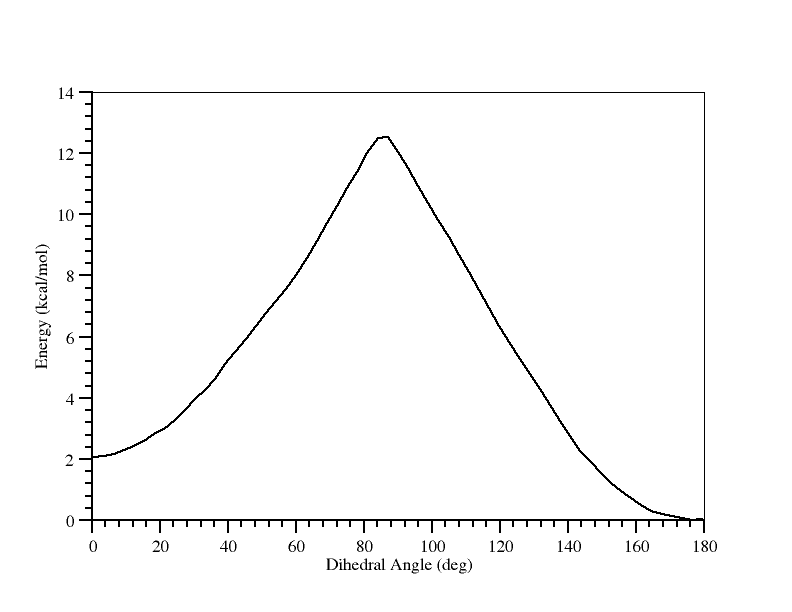
And there you have it. What this tells us is that the trans form is more stable than the cis form by approximately 1.8 kcal/mol and that the barrier to conversion from trans to cis is approximately 12.1 kcal/mol.

If you are feeling adventurous you could now try repeating this with QM/MM or even better try doing a simple reaction using QM/MM.

RETURN TO INDEX