Free energy calculations with the Free Energy Workflow (FEW) Tool
By Nadine Homeyer and Holger Gohlke
Please note: The workflow
tool FEW introduced here is
available in AmberTools 14 or any later version thereof and works with AmberTools and AMBER
version 14 or later. AmberTools and AMBER 14 can be installed by
following the installation guidelines given in the
AMBER manual. Bugfixes and new
source code will be automatically downloaded in the course of the
installation process.
This
tutorial is intended to demonstrate the functionality of FEW a workflow
tool for automated setup of free energy calculations for sets of
ligands binding to the same receptor. FEW allows to prepare
free energy calculations according to the molecular mechanics
Poisson-Boltzmann surface area (MM-PBSA), the molecular mechanics
generalized Born surface area (MM-GBSA), the linear interaction energy
(LIE), and the thermodynamic integration (TI) approach. Before using
FEW you should be familiar with running basic molecular dynamics (MD)
simulations in AMBER and with the theory and setup of the type of free
energy
calculation you wish to apply. Tutorials demonstrating setup and
execution of molecular dynamics simulations and free energy
calculations by the MM-PB(GB)SA and TI approaches can be found at
http://ambermd.org/tutorials. Explanations
of the theory of the free energy calculation
approaches are given in a number of reviews and books including:
MM-PB(GB)SA [1,
2],
LIE [3,
4],
and TI [5,
6].
In addition it is strongly recommended to read the article N.
Homeyer,
H. Gohlke, FEW - A Workflow Tool for Free Energy Calculations of Ligand
Binding. J. Comput. Chem.
2013, 34, 965–973. The sample free energy
calculations
shown in this tutorial, were selected from the case study described in
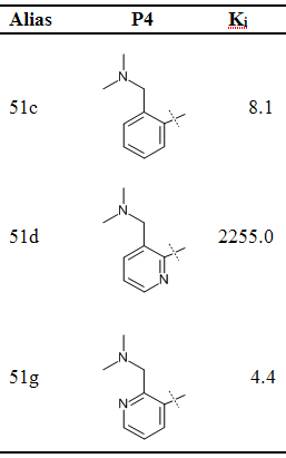
the article. We determine the relative binding free energies of 3
ligands (Table
1) that inhibit the protein Factor Xa, a protease playing an
important function in the blood coagulation cascade.
Required input structures:
- PDB structure of the receptor, i.e. the Factor Xa protein.
- Structures of
the ligands (in MOL2 format) with coordinates specifying the bound
position of the ligand.
If the binding mode of a ligand is not known, it can either be modeled based on the binding mode of similar ligands or obtained by docking programs. In the sample analysis shown here the former strategy was used. Please note that the expectable accuracy of the binding free energy predictions decreases with diminishing quality of the protein structure and the uncertainty of the ligand binding mode. Therefore only high quality protein (i.e. receptor) structures should be used and the binding position of the ligands should be modeled as exact as possible.
| Table 1: Ligand structures and experimentally determined Ki values in [nM] for Factor Xa |
 |
Preparatory work
To facilitate the reference to FEW in this tutorial, please set a variable $FEW to the path were FEW is installed on your system, e.g.:setenv FEW /home/src/FEW (for csh or tcsh) or
export FEW=/home/src/FEW (for bash, zsh, ksh, etc.)
If you type echo $FEW after defining the environment variable, the FEW installation path should be displayed.
The input files that will be used in this tutorial can be downloaded here. After unzippig and extracting the archive and following the installation instructions in the README file the files that are required for the tutorial should be located under $FEW/examples/tutorial.
Please create now a new folder and change into the new folder. In this tutorial we assume that the new folder is called tutorial and is located at /home/user/tutorial. You need to adjust the path according to the location of the folder on your system wherever it appears below.
Now copy the folders input_info (containing all required input files), structs (containing the ligand structures in Mol2 format), and cfiles (containing the command files for FEW) into the tutorial folder:
cp -r $FEW/examples/tutorial/input_info .
cp -r $FEW/examples/tutorial/structs .
cp -r $FEW/examples/tutorial/cfiles .
We have now all data we need in the local folder, so that we can start with the setup of the binding free energy calculations with FEW.
1. Setup of molecular dynamics (MD) simulations
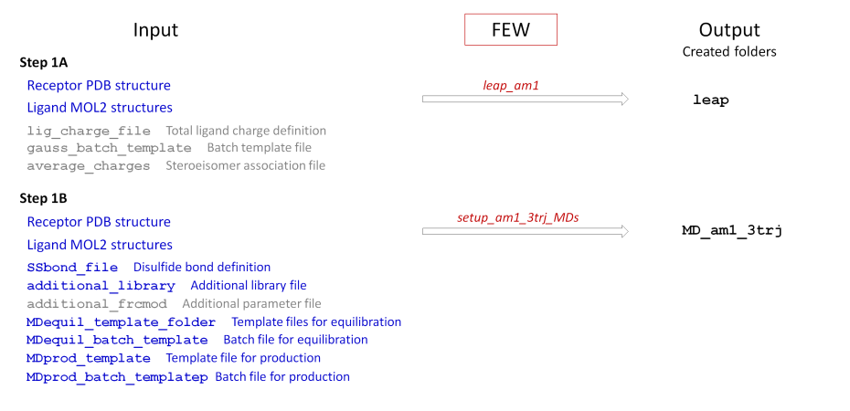
MM-PB(GB)SA and LIE calculations are conducted in FEW based on snapshots from MD simulations. Therefore this step needs to be executed before these types of free energy calculations are started. TI calculations can directly be started from crystal structures, but it is usually advisable to first run a short MD equilibration to remove bad contacts. Thus, only the latter alternative will be demonstrated here. For the former option please consult the FEW section of the AMBER manual.MD simulations are setup here in two steps, first the parameters for the ligands are determined (step 1A), then the input files for MD simulations are generated (step 1B). The two steps together with the required input information and the output generated by FEW are depicted in Figure 1.
Note:
In this tutorial for demonstration purposes simulations will be setup
for complex, receptor, and ligand (3-trajectory approach).
If you wish to conduct exclusively MM-PB(GB)SA calculations according
to the 1-trajectory approach (i.e. no LIE or TI calculations), it is
advisable to setup only complex simulations at this point.
 |
| Figure 1: Schematic depiction of setup of MD simulations with FEW. Input information used in this tutorial is highlighted in blue, input data that may be required for other systems / parameter settings are shown in gray, and command files for FEW are marked in red writing. Examples for input files not used here (gray in the scheme above) can be found in the folder $FEW/examples/input_info and an explanation of the required data format is provided in the FEW section of the AMBER manual. |
A: Preparation of parameter files
The setup of the MD simulations begins with the determination of the required parameters and the reformatting of the input structure files. For this we use the command file leap_am1 located in the folder /home/user/tutorial/cfiles.| leap_am1 |
| @WAMM ################################################################################ # Location and features of input and output directories / file(s) # # Location and features of input and output directories / file(s) # # lig_struct_path: Folder containing the ligand input file(s) # multi_structure_lig_file: Basename of ligand file, if multi-structure # file is provided # output_path: Basis directory in which all setup and analysis # folders will be generated # rec_structure: Receptor structure in PDB format # bound_rec_structure: Optional, alternative receptor structure in bound # conformation to be used for 3-trajectory approach lig_struct_path /home/user/tutorial/structs multi_structure_lig_file output_path /home/user/tutorial rec_structure /home/user/tutorial/input_info/2RA0_IN.pdb bound_rec_structure # Specification of ligand input format lig_format_sdf 0 lig_format_mol2 1 # Receptor features # water_in_rec: Water present in receptor PDB structure water_in_rec 1 # Request structure separation # structure_separation: Separate ligands specified in one multi-structure # input file and generate one structure file per ligand. structure_separation 0 ################################################################################ # Creation of LEaP input files # # prepare_leap_input: Generate files for LEaP input # non_neutral_ligands: Total charge of at least one molecule is not zero. # In this case the total charge of each non-neutral # molecule must be defined in lig_charge_file. # lig_charge_file: File with information about total charges of ligands. # am1_lig_charges: Calculate AM1-BCC charges. # resp_lig_charges: Calculate RESP charges. In this case charges must be # computed with the program Gaussian in an intermediate step. # Batch scripts for Gaussian calculations will be prepared # automatically, if requested (see prepare_gauss_batch_file # and gauss_batch_template below). # calc_charges: Calculate charges according to requested procedure. # If this flag is set to zero, no atomic charges are calculated. # resp_setup_step1: Step 1 of RESP charge calculation: Preparation of # Gaussian input. # resp_setup_step2: Step 2 of RESP charge calculation: Generation of LEaP input # from Gaussian output. # prepare_gauss_batch_file: Generate batch script for Gaussian input if RESP # charge calculation is performed. A batch template # file (gauss_batch_template) is required. # gauss_batch_template: Batch template file # Prerequisite: resp_lig_charges=1, resp_setup_step1=1 # and prepare_gauss_batch_file=1 # gauss_batch_path: Basic working directory for Gaussian jobs # average_charges: If the charges of two steroisomers shall be averaged, so that # both ligands obtain the same atomic charges, a file in which # the stereoisomer pairs are specified must be given here. prepare_leap_input 1 non_neutral_ligands 0 lig_charge_file am1_lig_charges 1 resp_lig_charges 0 calc_charges 1 resp_setup_step1 0 resp_setup_step2 0 prepare_gauss_batch_file 0 gauss_batch_template gauss_batch_path average_charges |
The leap_am1 file can directly be used as input command file for FEW. Only the basic input/output path marked in red needs to be adapted according to the location of the tutorial folder on your system. For clarity comments in the command file are shown in green above and only the key terms and the parameters are given in black writing.
In the first part of the file the parameters required for defining the general input and output data are specified. As we use single MOL2 structures in this tutorial, multi_structure_ligand_file does not need to be set. bound_rec_structure is also not specified, because we use only a single protein structure for both the complex bound and the free receptor in this setup. If the receptor structure changes its conformation upon ligand binding, two different receptor structures, one for the bound ( bound_rec_structure ) and one for the free state ( rec_structure), can be provided. The receptor structure we use here was derived from a crystal structure deposited in the Protein Data Bank as 2RA0. As the resolved crystal water molecules present in this structure were maintained and are specified as HOH residue entries in the provided receptor model structure (2RA0_IN.pdb), the water_in_rec flag is set to 1.
The second part of the command file comprises the parameters, required for the generation of the basic input files for LEaP. Here a calculation of atomic charges for the ligands by the AM1-BCC procedure is requested, therefore all parameters related to Gaussian calculations, that are required for calculation of atomic charges according to the RESP procedure, do not need to be provided. As furthermore all ligands are overall neutral (non_neutral_ligands=0), no lig_charge_file , in which the total charges of the ligands are defined, needs to be specified.
Running FEW:
After you changed the paths marked in red in the leap_am1 file above according to the location of your tutorial folder, the charge calculation and parameter preparation step can be started by:
perl $FEW/FEW.pl MMPBSA /home/user/tutorial/cfiles/leap_am1
The execution of this command can take about half an hour on a workstation machine, because the calculation of the atomic charges is computationally demanding.
The output:
When this first setup step was successfully terminated, a new folder called leap is present in the /home/user/tutorial directory. The leap folder contains a sub-folder for each ligand which comprises structure and parameter files required for setup of the MD simulations with LEaP.
Note: In this tutorial the simplest proceeding, i.e. the preparation of simulations with atomic charges determined by the AM1-BCC procedure, is demonstrated. If you wish to setup simulations with RESP charges, please consult the manual and use the example files $FEW/examples/command_files/commonMDsetup/leap_resp_step1 and $FEW/examples/command_files/commonMDsetup/leap_resp_step2.
B: Preparation of MD input files
The files for MD simulation input can be prepared with the command file setup_am1_3trj_MDs shown below. The color coding is the same as the one used in step 1A above.| setup_am1_3trj_MDs |
| @WAMM ################################################################################ # Location and features of input and output directories / file(s) # # lig_struct_path: Folder containing the ligand input file(s) # multi_structure_lig_file: Basename of ligand file, if multi-structure # file is provided # output_path: Basis directory in which all setup and analysis # folders will be generated # rec_structure: Receptor structure in PDB format # bound_rec_structure: Optional, alternative receptor structure in bound # conformation to be used for 3-trajectory approach lig_struct_path /home/user/tutorial/structs multi_structure_lig_file output_path /home/user/tutorial rec_structure /home/user/tutorial/input_info/2RA0_IN.pdb bound_rec_structure # Specification of ligand input format lig_format_sdf 0 lig_format_mol2 1 # Receptor features # water_in_rec: Water present in receptor PDB structure water_in_rec 1 ################################################################################ # Setup of molecular dynamics simulations # # setup_MDsimulations: Perform setup of simulation input # traj_setup_method: 1 = One trajectory approach # 3 = Three trajectory approach # MD_am1: Prepare simulations with AM1-BCC charges # MD_resp: Prepare simulations with RESP charges # SSbond_file: File with disulfide bridge definitions # additional_library: If an additional library file is required, e.g. for # non-standard residues present in the receptor structure, # this file must be specified here. # additional_frcmod: If additional parameters are needed, e.g. for describing # non-standard residues present in the receptor structure, # a parameter file should be provided here. # MD_batch_path: Path to basis directory in which the simulations shall # be performed in case this differs from <output_path>. # If no path is given, it is assumed that the path is # equal to <output_path> # MDequil_template_folder: Path to directory with equilibration template files # total_MDequil_time: Total equilibration time in ps # MDequil_batch_template: Batch template file for equilibration # MDprod_template: Template file for production phase of MD simulation # total_MDprod_time: Number of ns to simulate # MDprod_batch_template: Batch template file for MD production # no_of_rec_residues: Number of residues in receptor structure # restart_file_for_MDprod: Base name of restart-file from equilibration that # shall be used for production input setup_MDsimulations 1 traj_setup_method 3 MD_am1 1 MD_resp 0 SSbond_file /home/user/tutorial/input_info/disulfide_bridges.txt additional_library /home/user/tutorial/input_info/CA.lib additional_frcmod MD_batch_path MDequil_template_folder /home/user/tutorial/input_info/equi total_MDequil_time 400 MDequil_batch_template /home/user/tutorial/input_info/equi.pbs MDprod_template /home/user/tutorial/input_info/MD_prod.in total_MDprod_time 2 MDprod_batch_template /home/user/tutorial/input_info/prod.pbs no_of_rec_residues 290 restart_file_for_MDprod md_nvt_red_06 |
Input/Output information:
The part of the command file in which the parameters of the input and output data are specified is equivalent to the one shown in the preparation step 1A above. This part needs to be defined in all command files for FEW, regardless of the requested functionality. Otherwise FEW would not know where to locate and how to handle input files and where to write the output.
Setup
of MD simulations:
Simulations are prepared according to the 3-trajectory approach using
AM1-BCC
charges. Disulfide bridges
known to be present in the Factor Xa protein are specified in the
SSbond_file
called disulfide_bridges.txt
in
form of a tabulator separated
list of residue pairs connected by
disulfide
bonds. A library file
additional_library
is
provided for the structurally bound calcium ion present in the receptor
structure. Additional parameters are not required, since parameters for
calcium are available in the ff12SB force field, which is
used per default for the description of the receptor structure.
Equilibration: The
equilibration is prepared
using template files provided in the
equi
directory.
In the equilibration
procedure used here the molecular systems are first subjected to two
consecutive minimizations in which first high (min_ntr_h.in)
and
then low (min_ntr_l.in)
restraints
are applied to the solutes, i.e. the receptor and/or the ligand. In
case of the receptor all residues from 1 to
no_of_rec_residues
are
restrained.
After the minimizations MD equilibrations are performed with low
restraints on the solutes for a total of 400 ps. First the temperature
is raised to 300 K under NVT
conditions (md_nvt_ntr.in)
,
then the density is adjusted to 1 g/cm3
in a NPT simulation
(md_npt_ntr.in),
and
finally the restraints on the solutes are gradually removed in 50 ps
NVT
simulations
(md_nvt_red_<number>.in).
The
order in which the MD input files are processed is defined in the batch
script specified under
MDequil_batch_template.
If
you want to use a different equilibration procedure, you need to adjust
the
equilibration template files and the sander
calls in the batch file. However, usually the procedure applied here
should result in thoroughly equilibrated molecular systems.
(Template files for this equilibration procedure are also provided with
the FEW tutorial under
$FEW/examples/input_info/equi).
The
computing architecture specific settings in the
MDequil_batch_template
script generally need to be adapted
according to the requirements of your local computing facilities.
Please change only the first part
of the script until the statement
Fix
variables, if you want
to use the equilibration procedure described above.
Production: Input files for MD production are created based on the template file MD_prod.in such that the total production time amounts up to 2 ns. Please note, this short simulation time was chosen for demonstration purposes only. Usually much longer simulation times are needed to obtain a trajectory of a fully equilibrated state from which representative snapshots can be extracted. The basename of the final coordinate file from the equilibration restart_file_for_MDprod, used for MD production input, is md_nvt_red_06. The template batch file for MD production MDprod_batch_template needs to be adjusted before the Fixed variables statement and in the Re-queue section according to the computing architecture on which the MD simulations shall be run.
Running FEW:
After ensuring that the basic input/output path is correctly specified, the MD simulation setup can be invoked by calling FEW:
perl $FEW/FEW.pl MMPBSA /home/user/tutorial/cfiles/setup_am1_3trj_MDs
The output:
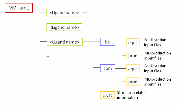
When the FEW run was successfully completed, a new folder called MD_am1 (Figure 2) is present in the basic input/output directory, i.e. the tutorial folder. As the name of the MD folder already tells, it contains files for running MD simulations with AM1-BCC charges. When you change into the MD_am1 folder, you see a sub-folder for each ligand and one for the receptor (rec). Every sub-folder contains a folder cryst in which the initial coordinate and topology files reside and the folders com (for complex) and lig (for ligand). The latter folders comprise the directories equi (with all files for MD equilibration) and prod (with the files for MD production) of the respective system.
 |
| Figure 2: Schematic depiction of substructure of MD folder created by FEW in step 1B. |
To start the MD equilibration, call the qsub_equi.sh shell script in the MD_am1 folder.
/home/user/tutorial/MD_am1/qsub_equi.shWhen the equilibration is complete for all ligands/complexes, start the production by calling the respective shell script in the MD_am1 folder.
/home/user/tutorial/MD_am1/qsub_MD.shNote: If you do not wish to run the MD simulations, you can copy the complete MD_am1 folder from $FEW/examples/tutorial/MD_am1 to your tutorial folder.
With the
trajectories from the MD simulations at hand,
it can be continued with the setup of the the free energy calculations.
Please click on one
of the links below, to get to the section, you are interested in.
SECTION 2: MM-PB(GB)SA calculations
Copyright: Nadine Homeyer 2014


