(Note: These tutorials are meant to provide illustrative examples of how to use the AMBER software suite to carry out simulations that can be run on a simple workstation in a reasonable period of time. They do not necessarily provide the optimal choice of parameters or methods for the particular application area.)
Copyright Ross Walker 2015

Analysis of water thermodynamics using Grid Inhomogeneous Solvation Theory of Factor Xa active site. SECTION 3

By Romelia Salomon, Crystal Nguyen, Steven Ramsey, Jonathan D. Gough, Ross Walker, & Tom Kurtzman

3) Analyzing the MD results with GIST

The final stage of our analysis is to use the cpptraj implementation of GIST to calculate the solvent structural and thermodynamic properties within a region of interest defined around the binding site of factor Xa.

As the name implies GIST (Grid Inhomogeneous Solvation Theory) will use a grid to define the region about which solvent properties are calculated. Therefore the first step is to define the region of interest using x y z coordinates. There are several ways that we could do this, common approaches involve picking a ligand atom as the center of the grid or visualizing a gridded region in a docking gui. Here we provide a helper script, FindCentroid.py, that when provided a ligand file will output a suggested GIST command that would define a gridded region of interest around the centroid of the provided ligand. Note: this helper script reads in any pdb structure file, as an example one could use it to define a region of interest centered on a particular protein residue by providing a pdb structure of that residue alone.

python FindCentroid.py -i 4QC.pdb

This code will output some information:

['4QC']
Centroid is:
(22.740924242424242, 28.46269696969696, 28.38016666666667)
Ranges are:
('x: ', 18.038, 27.65)
('y: ', 22.589, 33.676)
('z: ', 20.852, 36.274)
Recommended gist input command given input file (presumed ligand or binding cavity .pdb file)
gist gridspacn 0.5 gridcntr 22.741 28.463 28.380 griddim 48 55 77

This information describes the ligand and the coordinates that defines our region of interest and, in particular, outputs a cpptraj-gist command that would define this region of interest in the last line of output. Often expanding the region of interest to include a larger volume is necessary, here the script picks a size that is arbitrarily set to be roughly 5x the size of the ligand. In your work it may be appropriate to expand or shrink this region. NOTE: as the region of interest expands calculation runtime and memory usage increases, we recommend running a short GIST calculation (e.g. on the first 100 simulation frames) to estimate runtime and memory consumption, when time and memory are a concern.

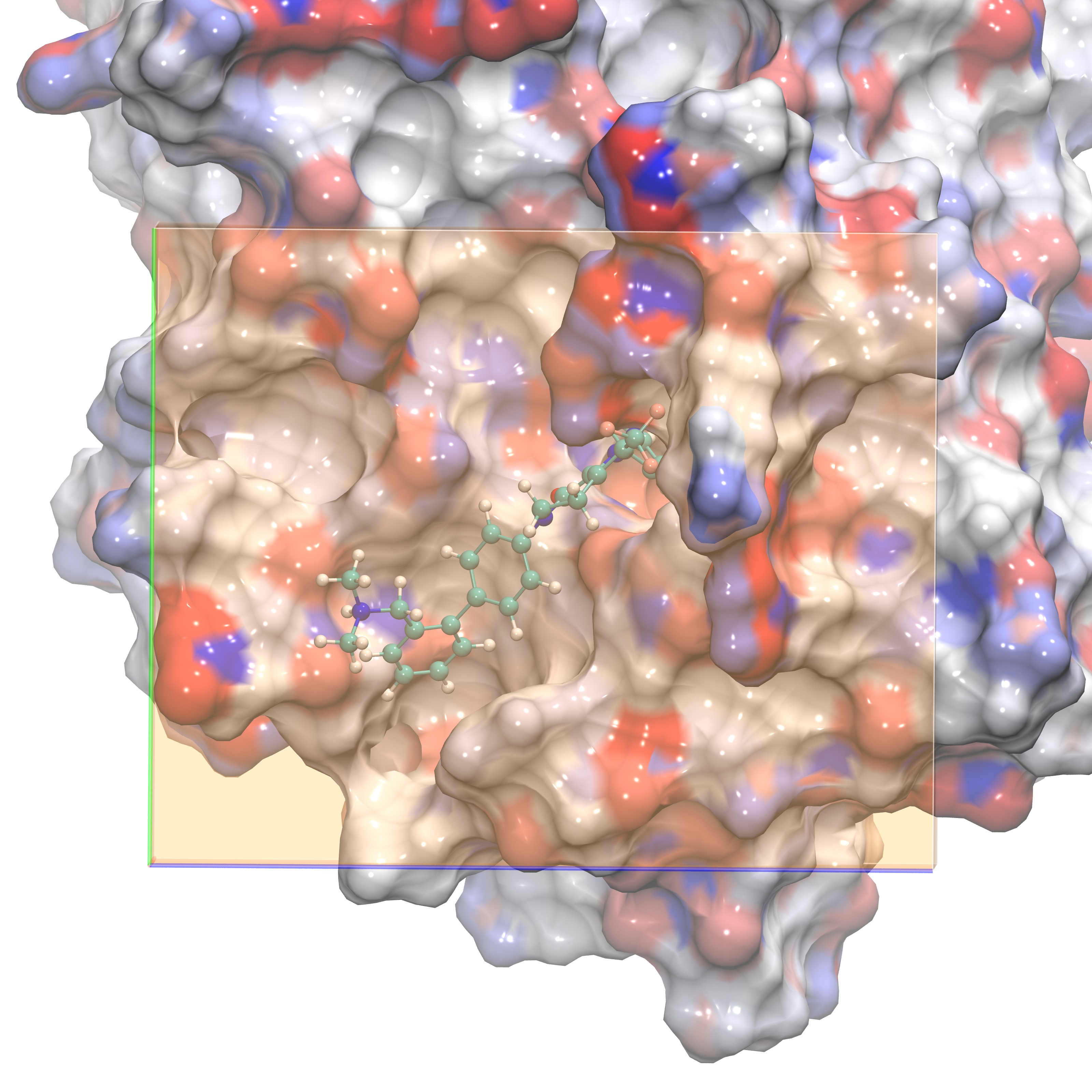
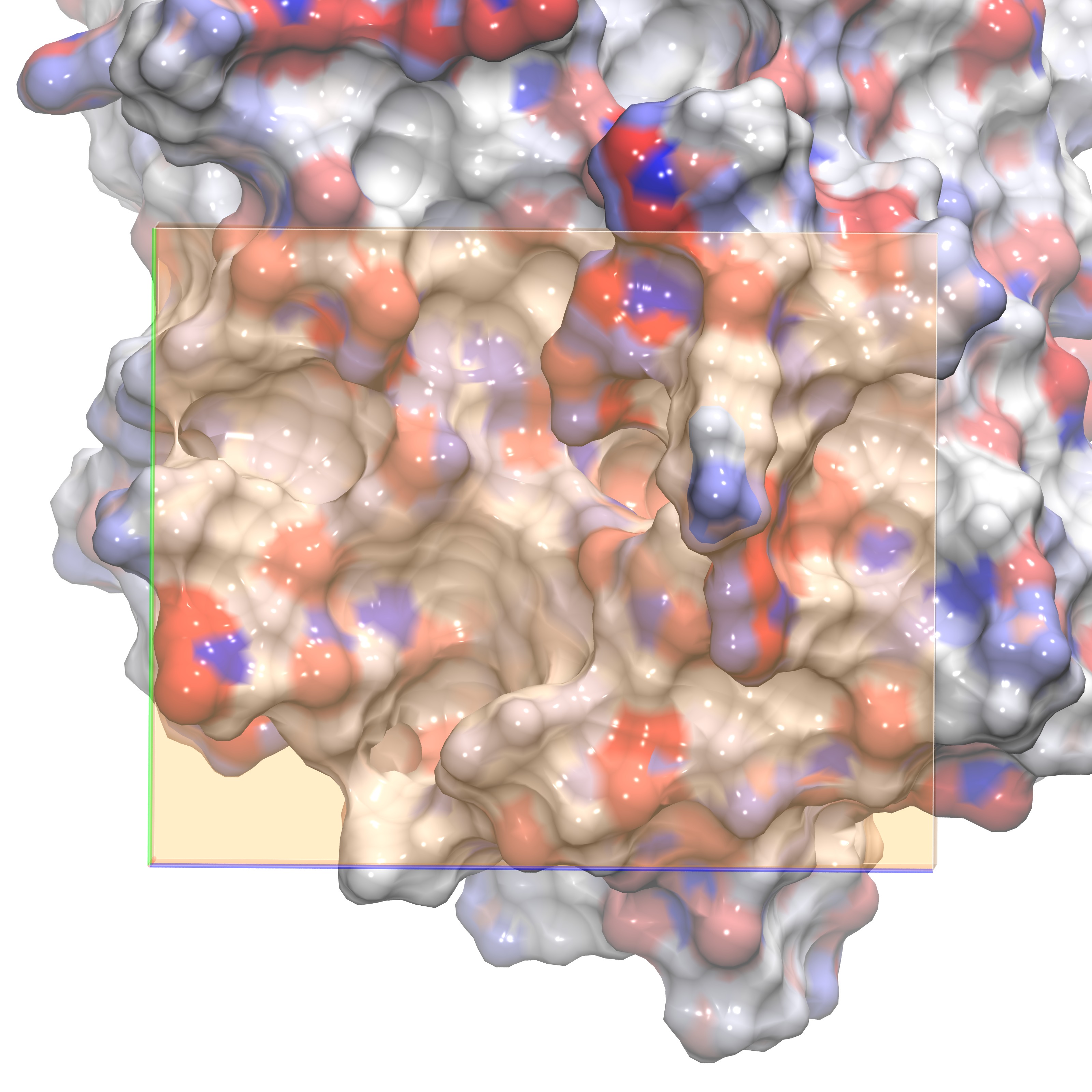
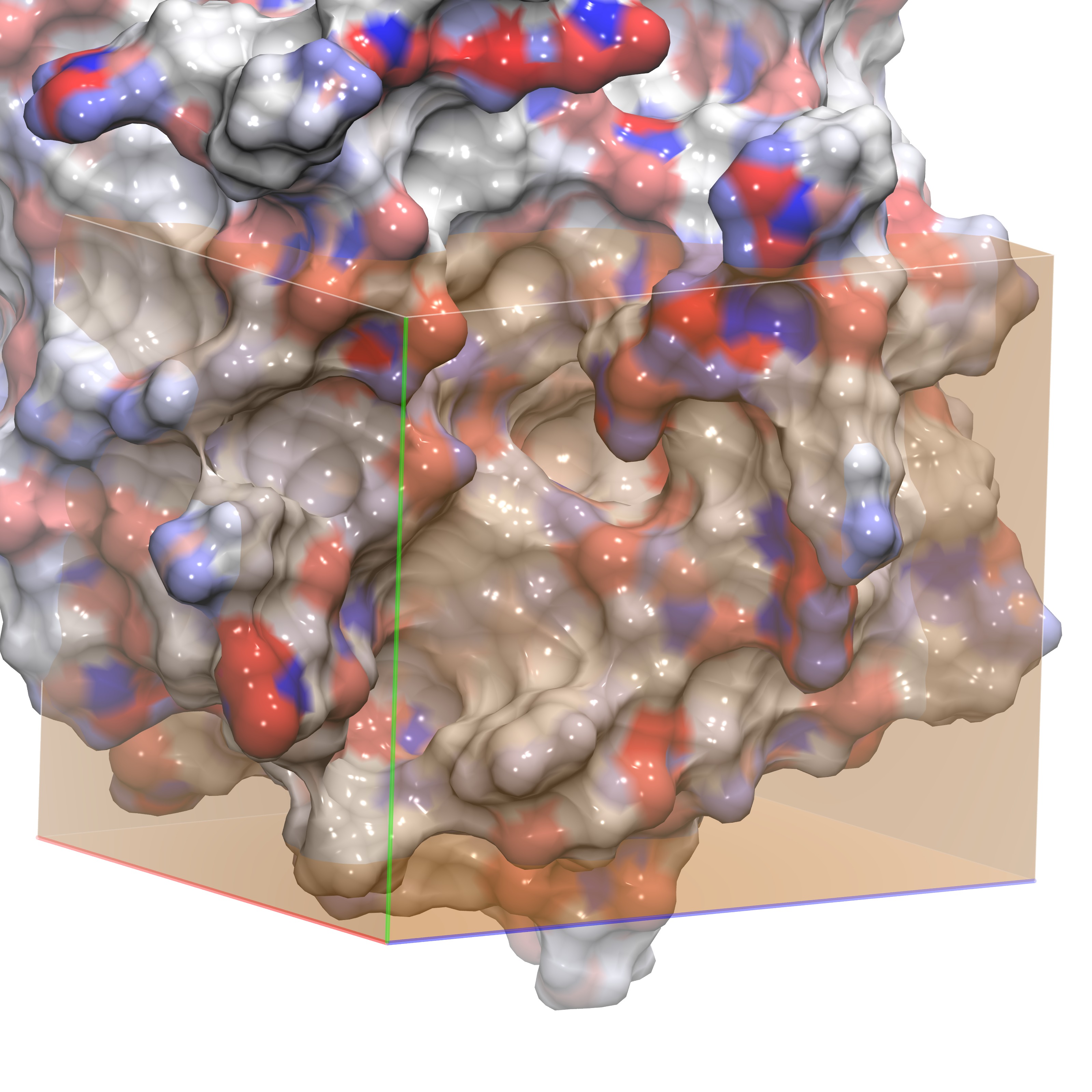
The following images show different views of the grid box employed for our GIST calculation. In order to understand the water structure within the ligand binding site, we define the GIST box so that it is placed exactly on top of the region where the ligand would bind. One option is to have a grid almost as large as the periodic box, however the user should be aware that this choice will make the GIST calculations much slower. See section 4f for details on helper scripts that will aid a user in performing GIST on a larger region of interest. The first figure shows the GIST grid with the ligand inside for visual aid. The last figure shows the box viewing the active site from the side.

Grid in front orientation plus ligand	Grid in front orientation without ligand	Grid in side orientation without ligand

For this tutorial it is assumed that you have downloaded and compiled cpptraj (contained within AmberTools) and know the basics of how to use it, if not please see the cpptraj AMBER Tutorial. Running GIST in cpptraj is as simple as running any other cpptraj Action command, requiring a parameter file (.prmtop), a trajectory file(.nc), and a few GIST specific arguments.

The cpptraj command for GIST with GIST specific arguments are as follows:

gist [doorder] [doeij] [refdens <rdval>] [gridcntr <xval> <yval> <zval>] [griddim <xval> <yval> <zval>] [gridspacn<spaceval>] [out <filename>]

The parameters that define the region of interest are as follows:

gridcntr: Coordinates (Å) of the center of the grid. The default values are (0.0,0.0,0.0).

griddim: Integer number of grid increments along each coordinate axis. The default values are (40,40,40).

gridspacn: Grid spacing (linear dimension of each voxel) in Angstroms. Values greater than 0.75 Å are not recommended, the default value is 0.5 Å .

NOTE: GIST calculation runtime scales with GIST region volume. Smaller regions will run more quickly, but it is important to define a region of interest that encompasses the full binding surface.

The other optional parameters provide additional thermodynamic and structural information, they are as follows:

doeij: Specifies if the triangular matrix representing the water-water interactions between pairs of voxels is calculated (default is false, not calculated).

doorder: Specifies whether the water order parameter will be calculated for each voxel (default is false, not calculated).

refdens: Specifies a reference density of bulk water, used in computing g_O, g_H, and the translational entropy. The default value is 0.0334 molecules/Å³.

NOTE: It is very important to ensure that refdens is appropriately set for the water model in use since all density quantities are relative to this reference bulk density.

The present implementation of GIST supports any 3-point and 4-point water model available in AMBER, here is a select list of these models:

a) TIP3P

b) TIP4P

c) TIP4PEW

d) OPC

e) TIP3PFW

f) SPCE

g) SPCFW

The AmberTools manual contains a full list of parameters and options available for GIST.

The simulation utilized in this tutorial is very simple, containing only the solute of interest and explicit waters. When performing GIST normally your production simulation may include other molecules, particularly ions. It is important that prior to GIST calculations you remove these ions from the simulation with the cpptraj command strip such that they are not included in the energy calculations performed by GIST. If ions are not removed they are considered part of the solute and will impact the calculated solute-water energy of interaction.

The trajectory is large and therefore the GIST calculation takes several hours.

For this analysis we use the following cpptraj commands:

parm fxa.prmtop
trajin prod_30ns.nc
gist gridspacn 0.5 gridcntr 22.670 28.524 29.551 griddim 48 49 60
go
quit

Simply, this script (gist.in) can be run as follows:

cpptraj -i gist.in &

As you will notice, a grid spacing value of 0.50 Å was employed. We do not recommend using values larger than 0.75 Å. Although, larger values will provide smoother results, the estimation of the thermodynamic values will be inaccurate. GIST is designed to have at most one water molecule per voxel for each frame.

In our example, GIST produces the file gist-output.dat, which provides all calculated quantities in a tabular format that can be imported into spreadsheet software, where each row corresponds to one grid box (voxel).

Below, we show the first three lines: the default comment, the column headers, and the first line of numerical output. The gist-output.dat file is a collection of all data produced by GIST printed in the order of grid point.

GIST Output, information printed per voxel

voxel xcoord ycoord zcoord population g_O g_H dTStrans-dens(kcal/mol/A^3) dTStrans-norm(kcal/mol) dTSorient-dens(kcal/mol/A^3) dTSorient-norm(kcal/mol) Esw-dens(kcal/mol/A^3) Esw-norm(kcal/mol) Eww-dens(kcal/mol/A^3) Eww-norm-unref(kcal/mol) Dipole_x-dens(D/A^3) Dipole_y-dens(D/A^3) Dipole_z-dens(D/A^3) Dipole-dens(D/A^3) neighbor-dens(1/A^3) neighbor-norm order-norm

0 15 21 19 415 0.994012 0.947305 0.000118875 0.00358058 0.000822792 0.0247829 0.000326025 0.00982002 -0.318998 -9.60836 0.00262741 -0.00135397 0.00170226 0.00341089 0.18016 5.42651 0

The first entries correspond to the voxel number followed by its x, y, z coordinates, while the next entries specify different values:

a) Population, atom density for oxygen and hydrogen (g_O and g_H).

b) Density weighted (dens) and normalized (norm) Translational and Orientational entropy: dTStrans-dens(kcal/mol/Å³), dTStrans-norm(kcal/mol), dTSorient-dens(kcal/mol/Å³) and dTSorient-norm(kcal/mol).

c) Density weighted (dens) and normalized (norm) Solute-water and water-water interaction energy: Esw-dens(kcal/mol/Å³), Esw-norm(kcal/mol), Eww-dens(kcal/mol/Å³), Eww-norm-unref(kcal/mol).

d) x, y, z dipole components, Dipole_x-dens(D/Å³), Dipole_y-dens(D/Å³), Dipole_z-dens(D/Å³), and the total dipole Dipole-dens(D/Å³).

e) Density weighted (dens) and normalized (norm) number of water neighbors within 3.5 Å of the voxel: neighbor-dens(1/Å³) neighbor-norm

f) Normalized tetrahedral order parameter, order-norm.

GIST produces a series of dx files in addition to the tabular output file, which contains all of the calculated data. These files can be readily visualized using VMD.

gist-dipole-dens.dx - Magnitude of mean dipole moment (polarization) (Debye/Å³).

gist-dipolex-dens.dx - X-component of the mean water dipole moment density (Debye/Å³).

gist-dipoley-dens.dx- Y-component of the mean water dipole moment density (Debye/Å³).

gist-dipolez-dens.dx - Z-component of the mean water dipole moment density (Debye/Å³).

gist-dTSorient-dens.dx - Density weighted first order orientational entropy (kcal/mole/Å³).

The more negative the isovalue, the more restricted or unfavorable the orientation of the water is. The value at bulk density is expected to be zero, most values will fall between 0 and -1.

gist-dTStrans-dens.dx - Density weighted first order tranlational entropy (kcal/mole/Å³).

The more negative isovalue, the more restricted the water is positionally. The value at bulk density is expected to be zero, most values will fall between 0 and -1.

gist-Esw-dens.dx - Density weighted Solute-Water interaction energy (kcal/mole/Å³).

This is the interaction of the water with the entire solute. Both Lennard-Jones and electrostatic interactions are computed without any cutoff, within the minimum image convention. The more negative the number, the more favorable the interaction between the water and solute is. Isovalues will be negative numbers.

gist-Eww-dens.dx - Density weighted Water-Water interaction energy (kcal/mole/Å³).

This is the interaction of the water with the entire solvent. Both Lennard-Jones and electrostatic interactions are computed without any cutoff, within the minimum image convention. The more negative the number, the more favorable the interaction between water within this voxel and all other water molucules is. Isovalues will be negative numbers.

gist-gH.dx - Number density of hydrogen centers found in the voxel, in units of the bulk density.

The expectation value of g_H for a neat water system is unity. The units of this dx file are the density/bulk density. Therefore an isovalue of 1 represents every voxel at or greater than bulk density.

gist-gO.dx - Number density of oxygen centers found in the voxel, in units of the bulk density.

The expectation value of g_O for a neat water system is unity. The units of this dx file are the density/bulk density. Therefore an isovalue of 1 represents every voxel at or greater than bulk density.

gist-neighbor-norm.dx - Mean number of neighboring water molecules, per water molecule found in the voxel (units of number per water).

Two waters are considered neighbors if their oxygens are within 3.5 Angstroms of each other.

gist-order-norm.dx - Average Tetrahedral Order Parameter for water molecules found in the voxel, normalized by the number of waters in the voxel.

doorder must be declared in the command line for this file to be produced.

All the information GIST produces allows for quantitative thermodynamic analysis of each voxel within the GIST region. Quantities are typically reported in a density-weighted format (weighted by water occupancy within a voxel). NOTE: normalized (average per water) values are not written to dx files by default, they are available in the gist-output.dat file. For more information on extracting these quantities see Section 4e in this tutorial).

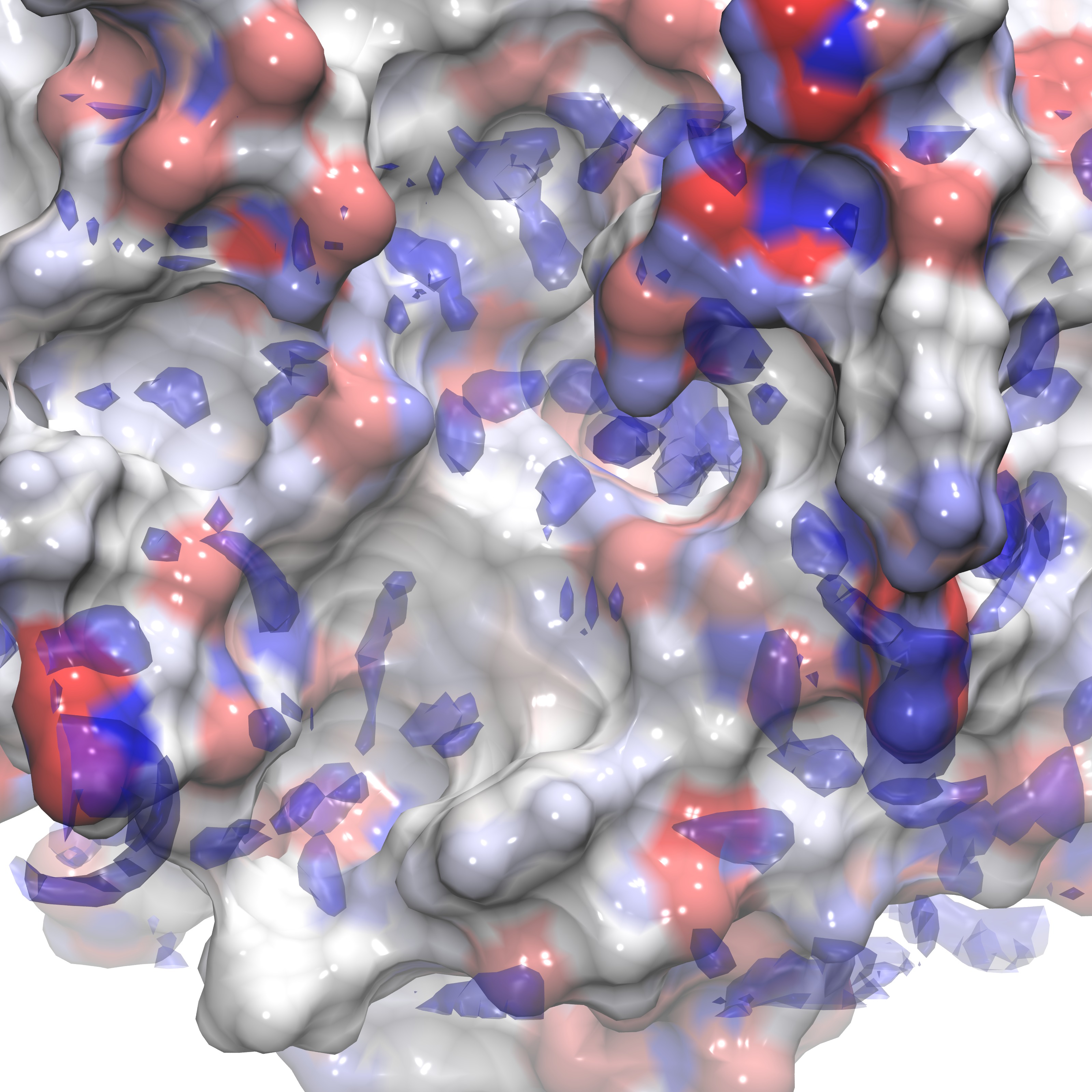
VMD can be used to visualize the dx files on the protein surface, to match the example figures below:

Load the protein structure, in this case you would load fxa.prmtop and final-prod.rst7 into that parmtop
Represent the protein structure with surf (or in our case MSMS -- a plugin downloaded from mgltools)
Color the protein surface by charge
Load a gist output data explorer (.dx) file as a new molecule in vmd
Represent said .dx file as show isosurface only, draw solid surface, and material transparent
By utilizing these settings these figures can be reproduced in vmd, note that we utilized white background, orthogonic perspective, and GLSL rendermode

These instructions can be utilized to produce a visualization similar to the figures below and can also be applied to any dx file output from Gist using isovalues appropriate for that .dx file (see above, or reference the figures presented below for examples).

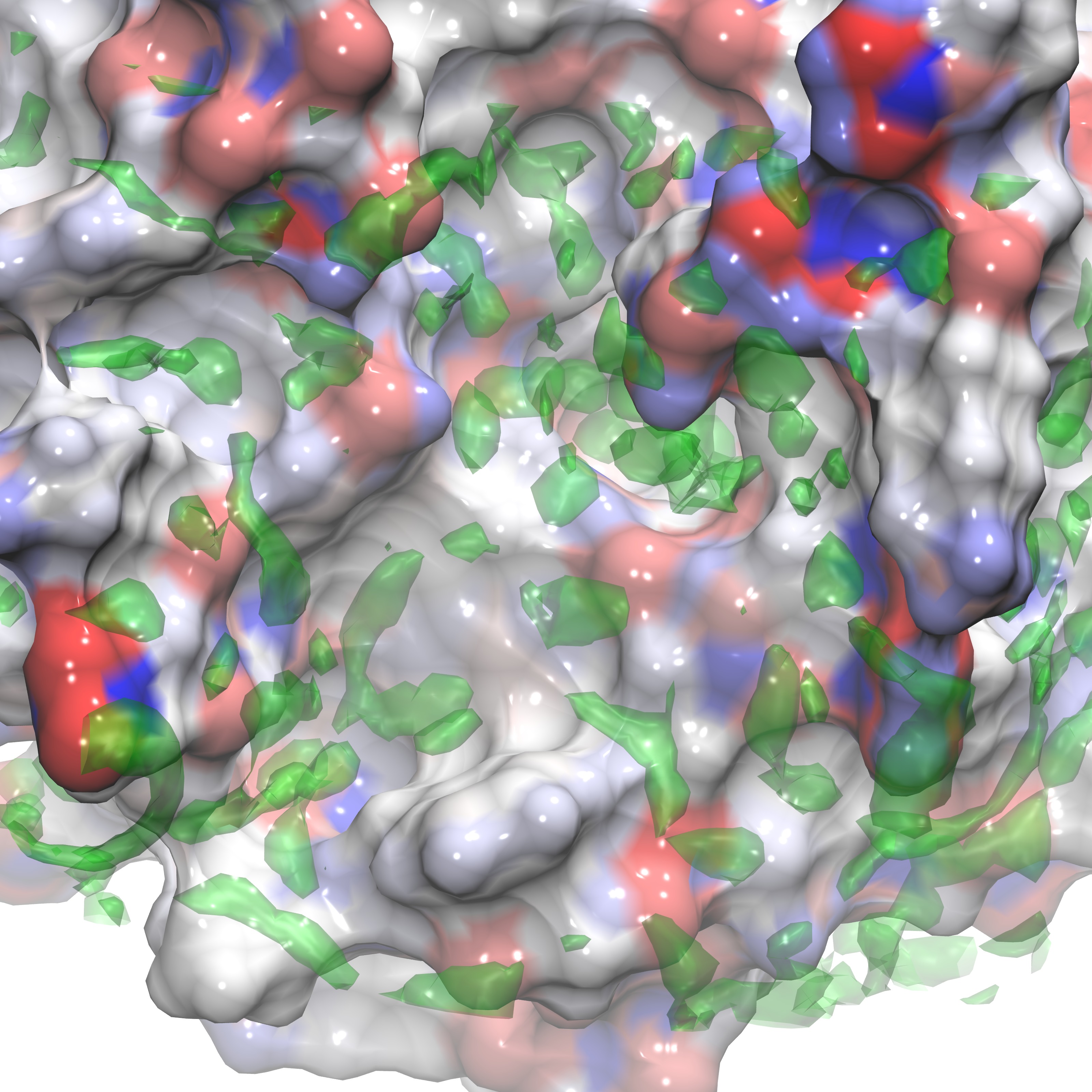
Here we show three representations of GIST data for three calculated quantites(gist-gO.dx g(O) green, gist-Esw-dens.dx E(sw) blue, and gist-dTStrans-dens.dx dTS(trans) purple) at specific isovalues (3.0,-0.7, and -0.1 respectively) on top of the electrostatic potential energy surface of the protein, in a blue-white-red scale.

If you are feeling adventurous you could now try repeating this with a longer simulation, like the one used in the paper [Nguyen et al.].

In the next section we review the use of various support tools that aid in evaluating GIST data.

CLICK HERE TO GO BACK TO SECTION 2 CLICK HERE TO GO TO SECTION 4