(Note: These tutorials are meant to provide illustrative examples of how to use the AMBER software suite to carry out simulations that can be run on a simple workstation in a reasonable period of time. They do not necessarily provide the optimal choice of parameters or methods for the particular application area.)
Copyright Ross Walker 2015

Analysis of water thermodynamics using Grid Inhomogeneous Solvation Theory of Factor Xa active site. SECTION 4

By Romelia Salomon, Crystal Nguyen, Steven Ramsey, Jonathan D. Gough, Ross Walker, & Tom Kurtzman

4) Analyzing GIST data with GISTPP

In this section GIST output data will be processed with GISTPP (gist post processing) a software suite which contains several useful operations that can be applied to GIST data. This section will not provide a full breakdown of GISTPP functionality, for that please reference its standalone manual (published in the future). Rather this section will focus on specific applications that should produce potentially useful data (and demonstrate the majority of GISTPP functionality in an application context). The applications below include calculating a solvent accessible surface area (SASA), performing numerical operations with GIST output, integration over solvent volumes in the context of comparing ligand poses, grouping solvent data based on similarity and proximity, and using GISTPP to produce a dx file from any of the data calculated during GIST which does not typically produce a standalone dx file.

At this stage it is assumed that the previous steps have come to completion successfully and the standard GIST output files are present (such as: gist-gO.dx, gist-Eww-dens.dx, etc.). The files used in this section can be found here: gist-gO.dx, gist-Eww-dens.dx, gist-Esw-dens.dx, gist-dTStrans-dens.dx, gist-dTSorient-dens.dx, and gist-output.dat.

Also of interest are two different ligands that bind this system, structure files for these can be found here: RRR.pdb, 4QC.pdb.

4a) Compiling GISTPP

Before getting into how GISTPP works and example applications the source code can be found in the GISTPP git repository here: github. It can be compiled with gcc compilers for C++ on most linux (and mac) machines with the command:

g++ -o gistpp gistpp.cpp gistpp_main.cpp

Usage instructions for GISTPP are as follows:

./gistpp -i infile -op operation [-i2 infile 2][-o outfile][-opt options]
where:
bracketed commands are either optional or required dependant on the operation to be performed
infile is a file containing the main data to be read, this can either be the gist output file or a dx file
operation is the required specification of a desired operation to be performed on the infile
To see a full list of operations run: ./gistpp -operation
[infile 2] is a second infile, necessary when using an operation which requires two input files (ex: add or clear2)
[outfile] is the desired name of an outfile if the operation performed produces an outfile. Default is out.dx
[options] are various option flags which apply to specific operations
To see a full list of options and the operations they apply to run: ./gistpp -options

For help instructions related to running GISTPP:

Execution help can be seen by running: ./gistpp or ./gistpp -h
Operation details can be seen by running: ./gistpp -operation
Option details can be seen by running: ./gistpp -options

4b) Generating the Solvent Accessible Surface Area (SASA)

The solvent accessible surface area (SASA) of a protein is the surface that describes the most proximal voxels to the protein at which water oxygen's were found during the simulation. This surface effectively describes the ligand accessible area as well since ligand heavy atom vdw radius will be similar to that of oxygen. The algorithm that finds SASA voxels searches each voxel to determine whether water was present (g_O > 0.3) and has at least one neighboring voxel in which water was not present (g_O < 0.1). To produce a SASA the only input required is the gist-gO.dx produced in the previous section. The command is:

./gistpp -i gist-gO.dx -op sasa -o SASA.dx

The following plots represents the SASA.dx produced when this command is executed, represented in transparent surface shown from the front and side.

4b) Performing numerical combinations on GIST output with GISTPP

GIST output can be extremely helpful in exploring solvent properties on a protein surface, however the default output alone can be difficult to analyze directly. To compensate GISTPP has a few operations that allow users to manipulate GIST output data to represent, in a more clear fashion, whatever information is pertinent. For a full list of operations refer to the GISTPP manual file included in its git repository. As an example here we will produce dx files that represent total solvent energy, total solvent entropy, and solvent free energy. First we will produce a dx file that contains total solvent energy with the following commands:

./gistpp -i gist-Esw-dens.dx -op multconst -opt const 0.5 -o half-gist-Esw-dens.dx

./gistpp -i gist-Eww-dens.dx -i2 half-gist-Esw-dens.dx -op add -o gist-Etot-dens.dx

./gistpp -i gist-Etot-dens.dx -op multconst -opt const 0.125 -o gist-Etot.dx

The first command will devide the solvent-solute interaction energy by 2 (of note, the Eww,water-water interaction energy, has been divided by 2 in the code already). The second command will take the two solvent energy dx files produced during GIST and add them together voxel by voxel, so that the resulting output file contains voxel data of their combination (solute-water + water-water energetic contributions = total energy). Once done these data remains density weighted which can be removed through the second command which reads in gist-Etot-dens.dx and multiplies each voxel by a constant (the volume of the voxel in this case) to modify the data from an energy density to total energy.

From here in order to calculate free energy we require a temperature weighted entropy quantity as well, however again GIST output's entropy as two separate files: gist-dTStrans-dens.dx and gist-dTSorient-dens.dx. Therefore we must combine them first, remove the density weighting as above. These commands are shown below:

./gistpp -i gist-dTStrans-dens.dx -i2 gist-dTSorient-dens.dx -op add -o gist-dTStot-dens.dx

./gistpp -i gist-dTStot-dens.dx -op multconst -opt const 0.125 -o gist-dTStot.dx

Finally we must combine these files to create a solvent free energy dx file, to do so we simply subtract dTStot from Etot (A = E – TS):

./gistpp -i gist-Etot.dx -i2 gist-dTStot.dx -op sub -o gist-dA.dx

4c) Integration of solvent quantities over ligand pose volumes

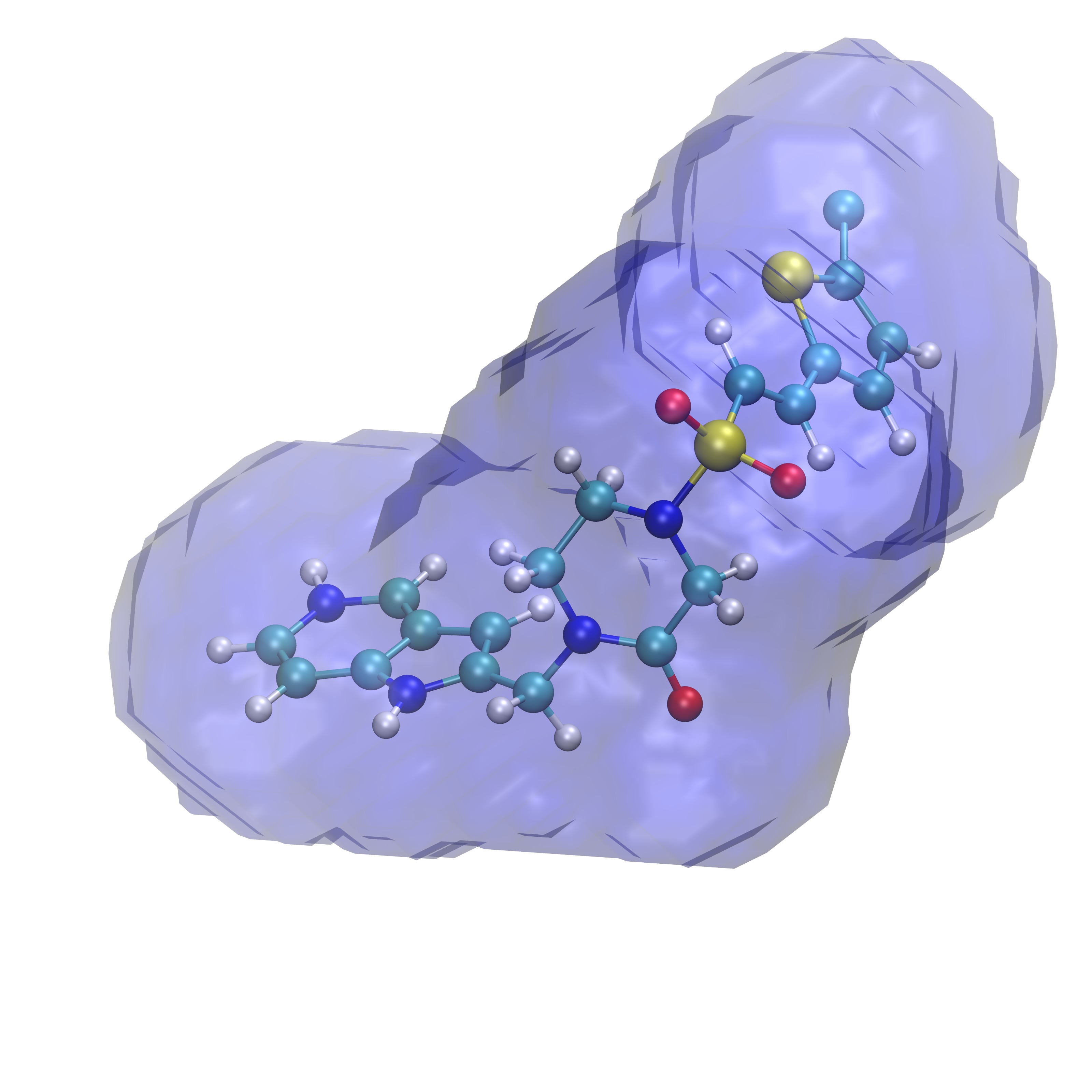
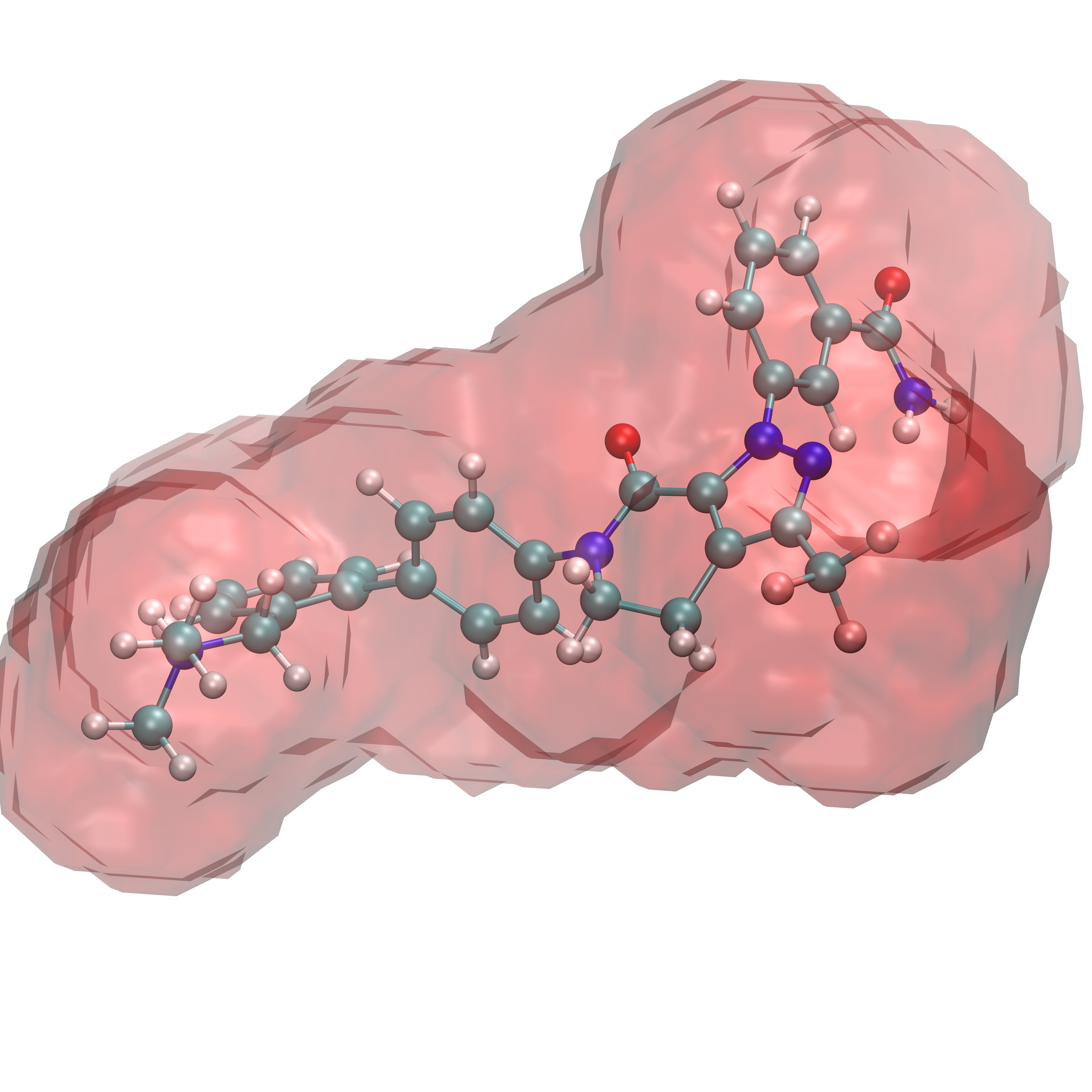
Comparing ligand poses based on the expulsion of water can be incorporated into determining pose viability. To do so one would need to be able to calculate the properties of the solvent that would likely be displaced by a pose of interest. In order to do so GISTPP has several operations designed to tackle this task. First the volume around a ligand must be defined in order to estimate the volume of water that will be expelled from the binding surface. For this tutorial we will utilize the two ligands: RRR.pdb and 4QC.pdb. To define the volume around their binding pose we will first one the GISTPP operation defbp (define binding pose) with both ligands:

./gistpp -i gist-gO.dx -i2 RRR.pdb -op defbp -opt const 3 -o bp3_RRR.dx

./gistpp -i gist-gO.dx -i2 4QC.pdb -op defbp -opt const 3 -o bp3_4QC.dx

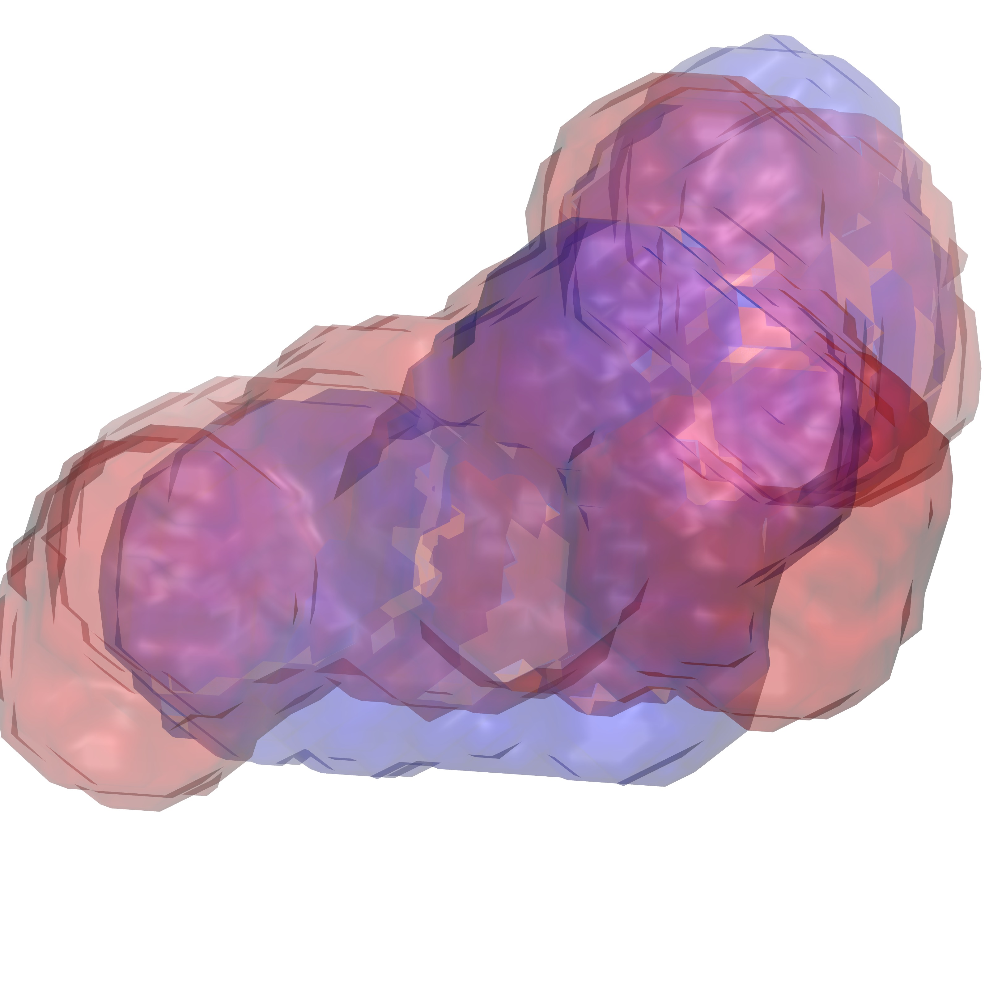
In this command '-opt cutoff1 3' defines the volume of interest for us is within 3 Å of any ligand heavy atom. Below are figures representing the output files produced from this step:

Though interesting to see how the two ligand volumes compare visually it may be useful to compare the water thermodynamic quantities found within those volumes. To do so we will multiply the output files bp3_RRR.dx and bp3_4QC.dx by the thermodynamic files we produced previously in this section. The reason we can multiply them together is that each of the binding pose dx files contains 1's in each voxel within the region of interest and 0's in voxels outside it. Therefore when each file is multiplied with say gist-Etot.dx the voxel will contain 0 when outside the region and whatever energy it contains if within the volume. To produce these files we will perform three multiplications on each binding pose with the following commands:

./gistpp -i bp3_RRR.dx -i2 gist-Etot.dx -op mult -o RRR3_Etot.dx

./gistpp -i bp3_RRR.dx -i2 gist-dTStot.dx -op mult -o RRR3_dTStot.dx

./gistpp -i bp3_RRR.dx -i2 gist-dA.dx -op mult -o RRR3_dA.dx

./gistpp -i bp3_4QC.dx -i2 gist-Etot.dx -op mult -o 4QC3_Etot.dx

./gistpp -i bp3_4QC.dx -i2 gist-dTStot.dx -op mult -o 4QC3_dTStot.dx

./gistpp -i bp3_4QC.dx -i2 gist-dA.dx -op mult -o 4QC3_dA.dx

After these steps we have 6 files, 3 for each ligand pose. These files contain the Etot, dTStot, and dG quantities for the voxels within the ligand pose volume respectively. In order to determine the relative difference between each pose however we would need to integrate over that volume for each ligand. To do so we will use a GISTPP operation called 'sum' which will sum the quantities within a specified dx file and print the total in the command line interface. The commands to do so are as follows:

./gistpp -i RRR3_Etot.dx -op sum

./gistpp -i RRR3_dTStot.dx -op sum

./gistpp -i RRR3_dA.dx -op sum

./gistpp -i 4QC3_Etot.dx -op sum

./gistpp -i 4QC3_dTStot.dx -op sum

./gistpp -i 4QC3_dA.dx -op sum

The output values should appear as follows:

sum of: RRR3_Etot.dx is: -295.557

avg of: RRR3_Etot.dx is: -0.00209437

sum of: RRR3_dTStot.dx is: -50.3386

avg of: RRR3_dTStot.dx is: -0.000356708

sum of: RRR3_dA.dx is: -245.218

avg of: RRR3_dA.dx is: -0.00173766

sum of: 4QC3_Etot.dx is: -333.162

avg of: 4QC3_Etot.dx is: -0.00236084

sum of: 4QC3_dTStot.dx is: -55.8619

avg of: 4QC3_dTStot.dx is: -0.000395847

sum of: 4QC3_dA.dx is: -277.3

avg of: 4QC3_dA.dx is: -0.001965

NOTE: The average reported after each sum is not useful information in this context as it is the average of the values in all voxels, these files contain a large number of voxels with a value of 0 (not a part of the ligand region) therefore the average is not restricted to voxels of interest.

4d) Creating groups based on solvent properties

Computational studies that seek to utilize solvent properties often require locating regions that contain specific solvent thermodynamics or structural properties. As an example locating volumes that contain solvent with high (unfavorable) energy can be used to predict regions amenable to ligand insertion. It is possible to visualize GIST energy output (such as gist-Eww-dens.dx) and contour the dx file in VMD to only represent regions with high energy and determine these locales manually, however it may be simpler to utilize operations present in GISTPP to produce groups of high energy regions. Utilizing GISTPP also allows integrating said groups to determine which groups are the most unfavorable, and extrapolate to predictions of ligand affinity changes upon expulsion. In this example it is most useful to group together regions that contain high solvent density (g_O) and high solvent energy in order to find volumes proximal to the ligand pose tractable for ligand modifications. First we will produce a dx file that contains data in voxels that meet the criteria of both high solvent density and energy:

./gistpp -i gist-gO.dx -i2 gist-Etot.dx -op filter2 -opt cutoff1 2.0 -opt gt1 -opt cutoff2 -0.25 -opt gt2 -o highGhighE.dx

This command utilizes the operation in GISTPP 'filter2'. Filter2 reads in two dx files and produces a third which contains 1's in each voxel which meets the criteria's applied to both input files. In this case we specify g_O greater than 2 (-opt cutoff1 2.0 -opt gt1) and Etot greater than -0.5 (-opt cutoff2 -0.5 -opt gt2). If one were interested in creating a criteria of less than some cutoff the flag would be 'lt1' or 'lt2' (ex: -opt cutoff1 2.0 -opt lt1). Note the options specified with -opt apply input file specified in the option (i.e. cutoff1 applies to -i, the first file). The created file should appear as the figure below:

At this point we have created a file that contains flags (remember the output is in binary: 1 for yes, 0 for no) in voxels that contain high density and high E. From here we have a reasonable file to utilize GISTPP's grouping operation. This operation expects a binary format in that it merely groups non zero voxels based on spatially proximity, therefore this operation will not produce meaningful results from a default energy output file. The command to create groups from our file is as follows:

./gistpp -i highGhighE.dx -op group

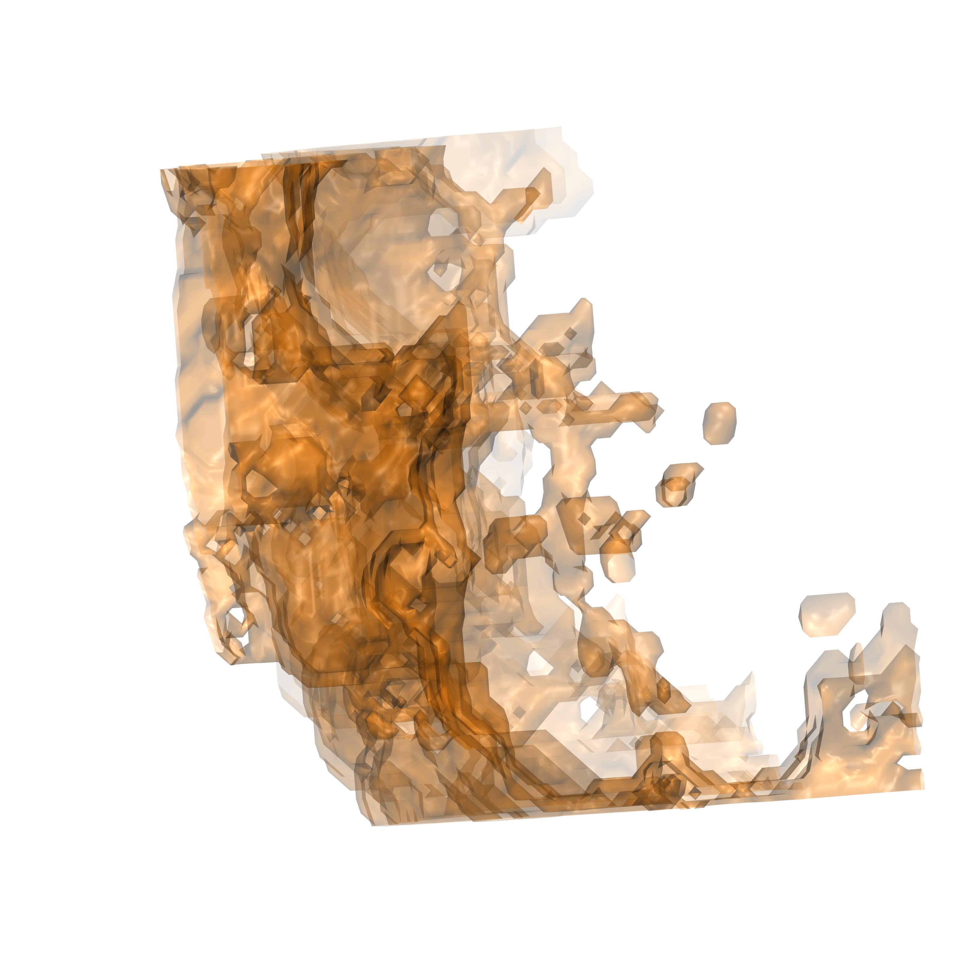
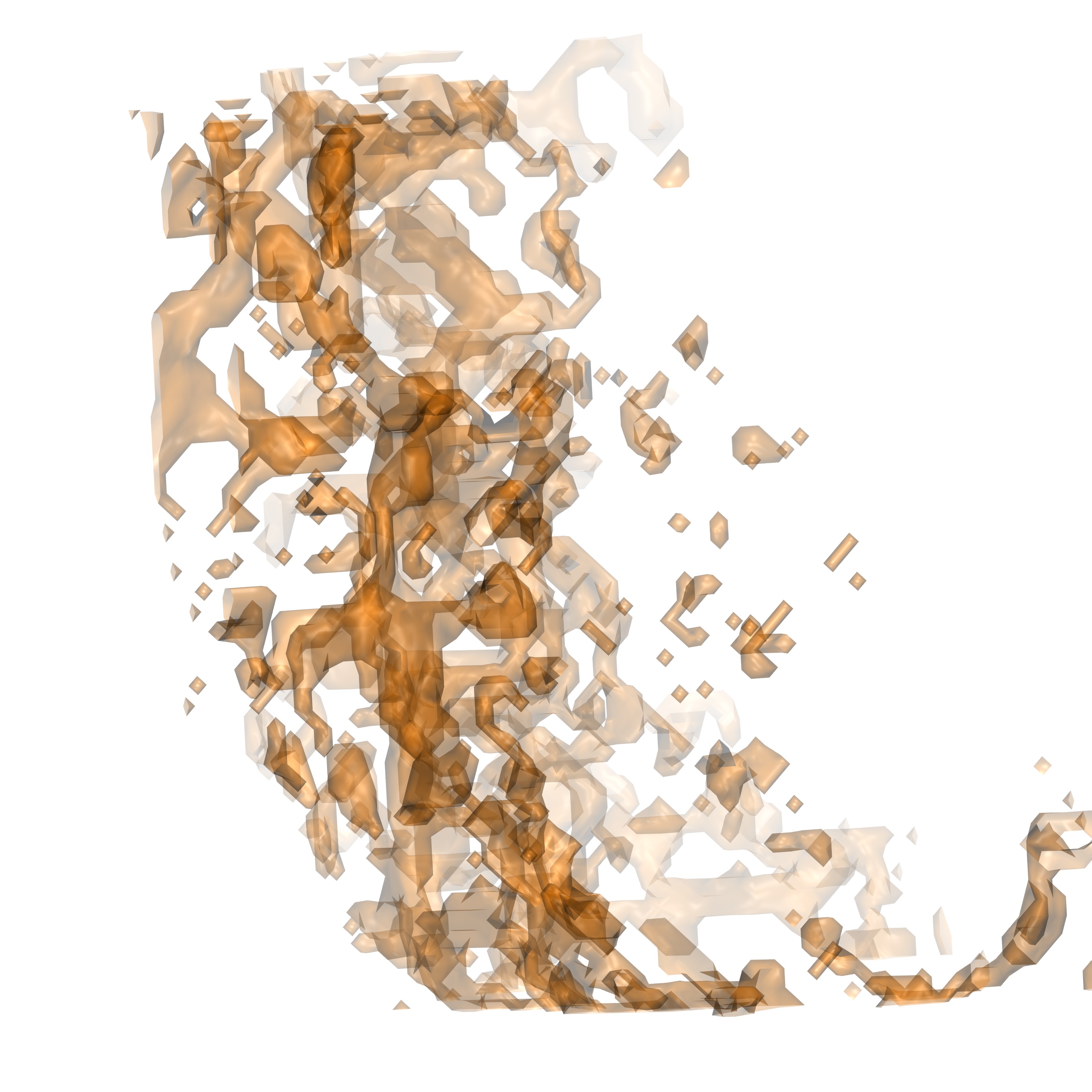
This command will produce several files: mastergroup.pdb, mastergroup.dx, grcount.txt, and group1.dx to group171.dx. These files contain various data, mastergroup's contain all groups together, the pdb file is especially useful as each groups number is stored in resid, which allows the user to visualize all groups and determine specific groups of interest. The file grcount.txt contains a list of all groups and their voxel occupancy. Each group.dx file contains that specific group. Below are a few representations of the produced groups

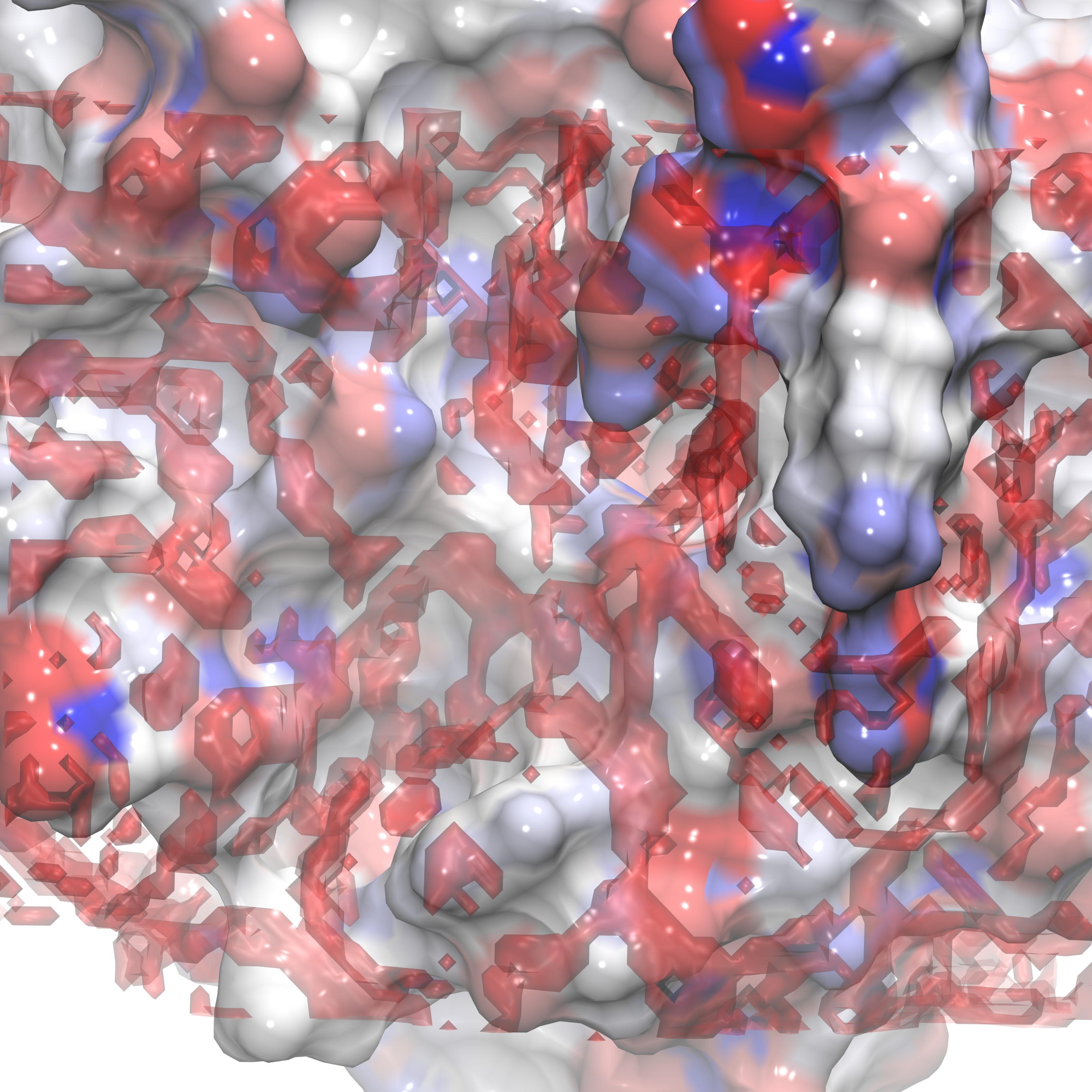
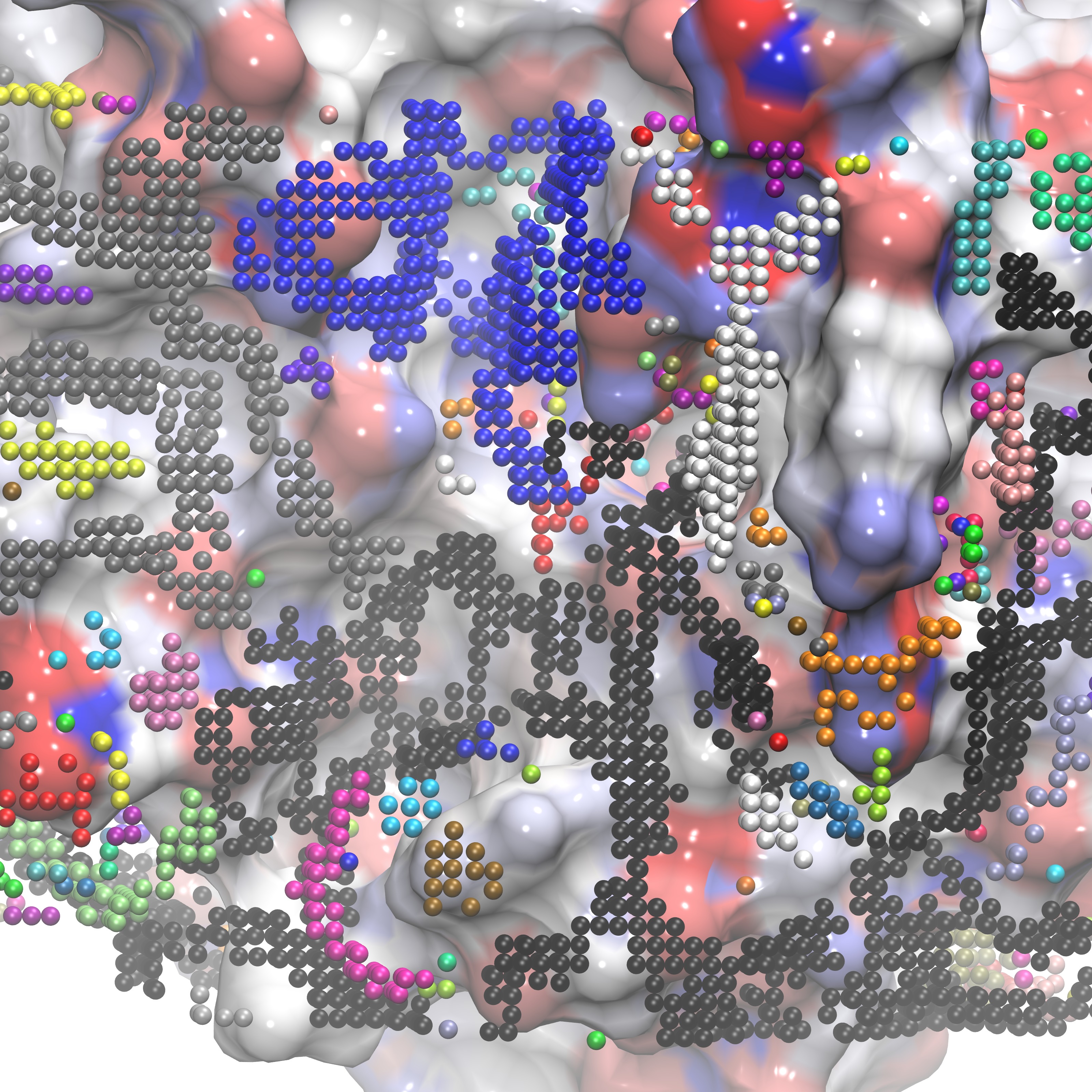
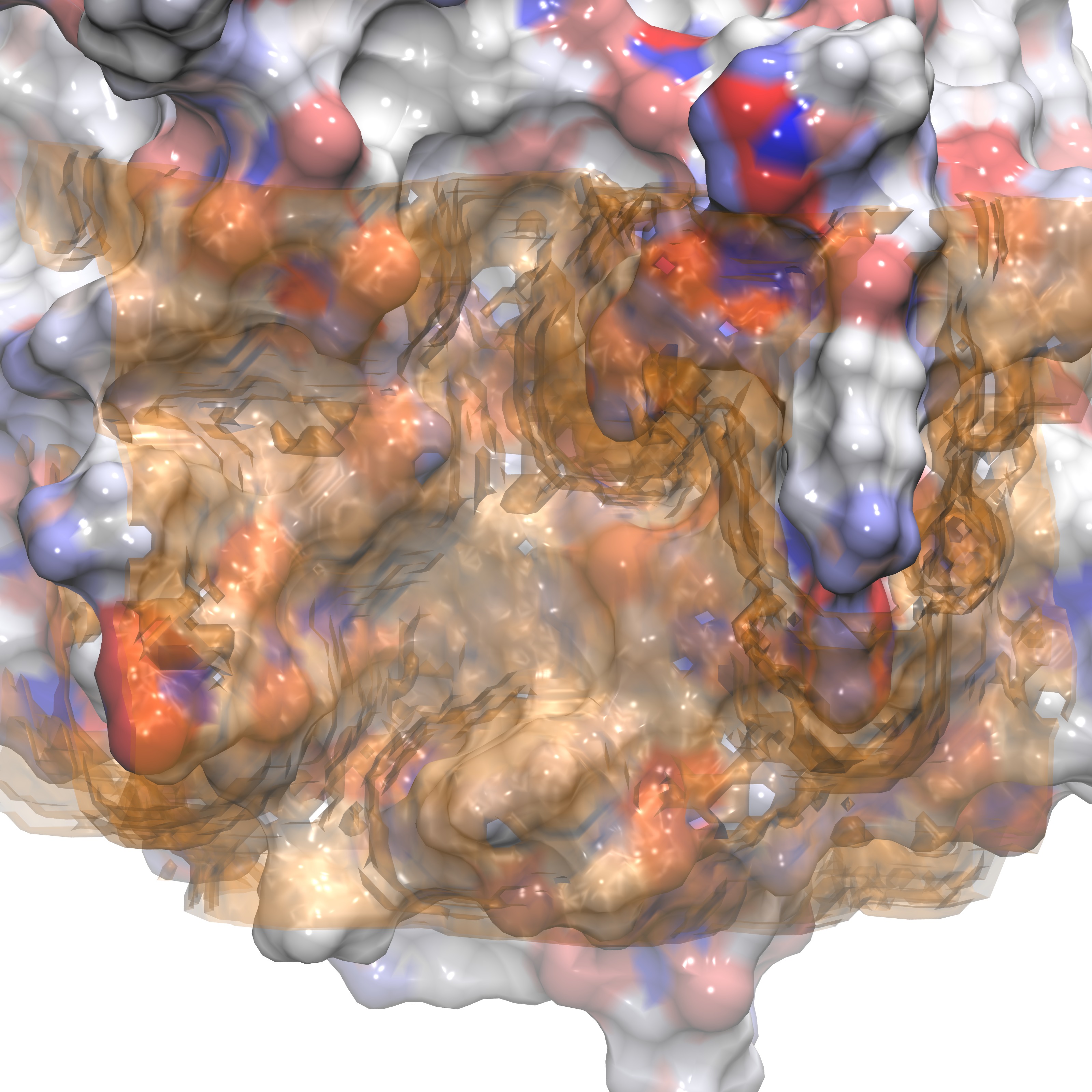
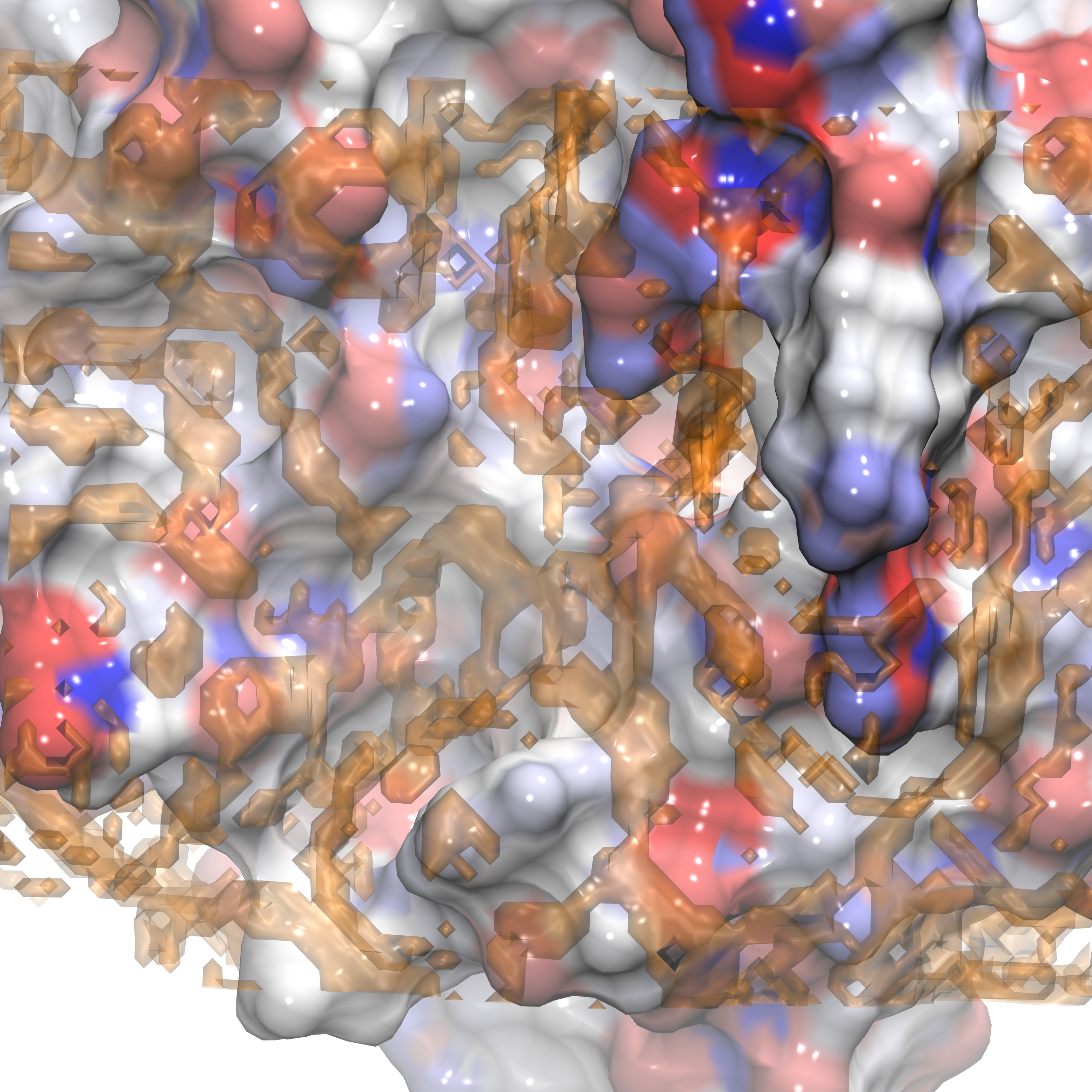
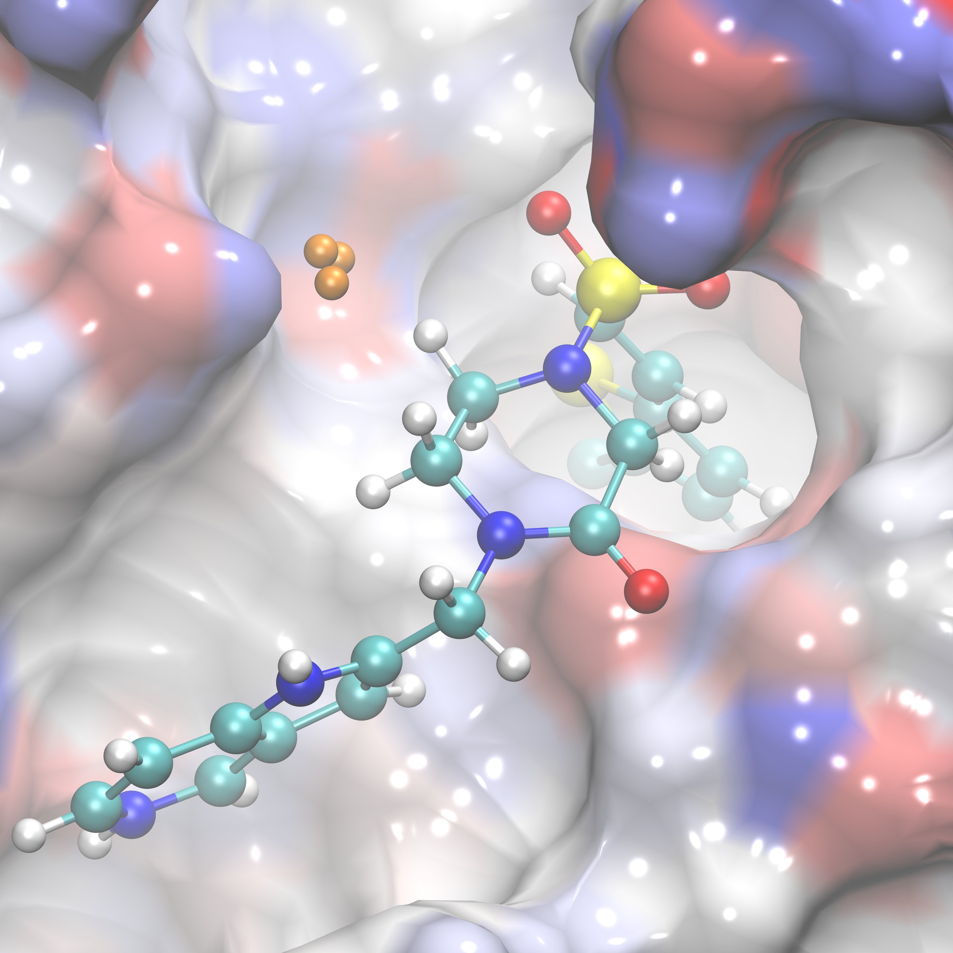
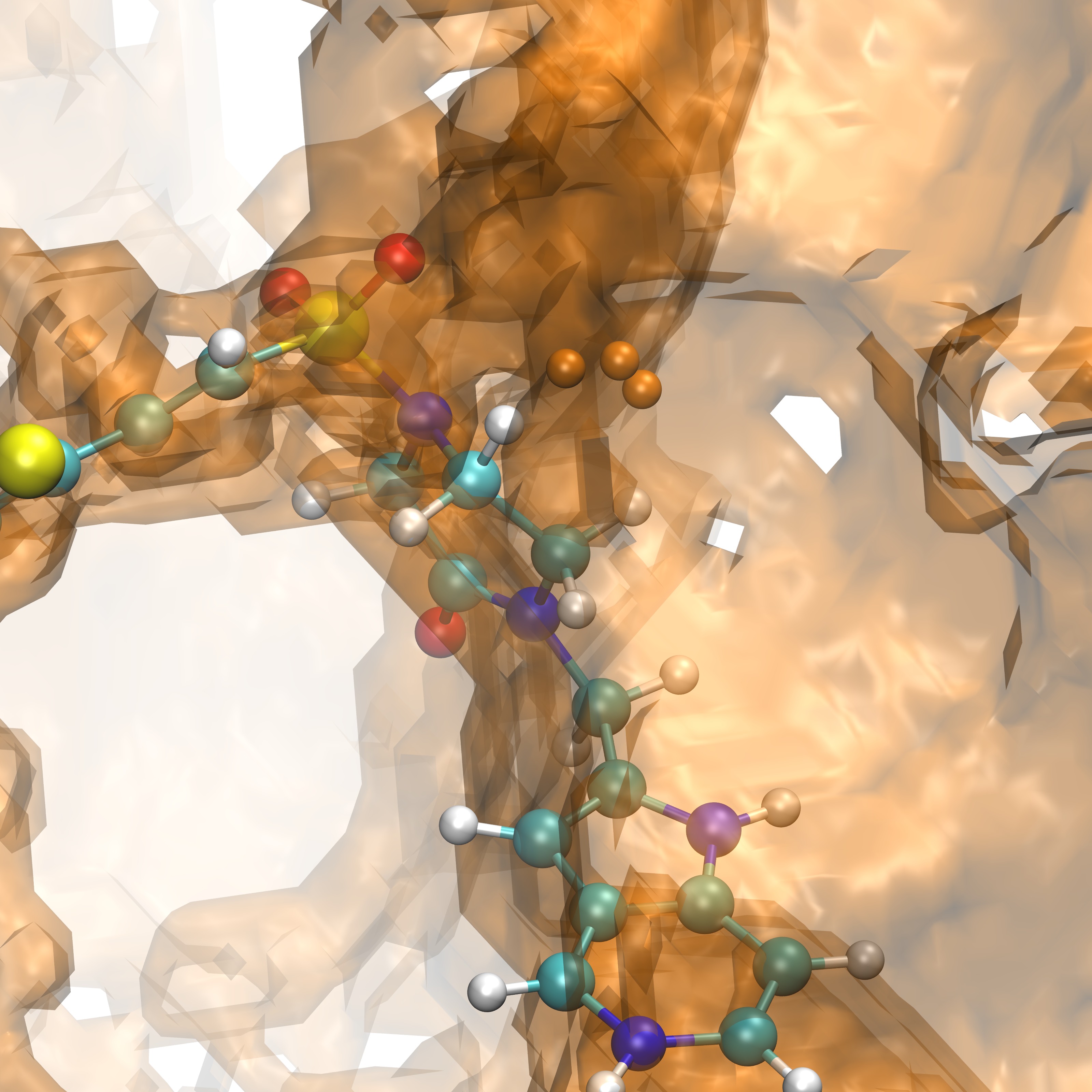
We can now identify groups that are proximal to our ligand RRR.pdb within VMD, shown below is the selection of group 25:

Once groups that are proximal to our ligand, but not overlapping with the ligand have been identified such as group 99 shown above we can then analyze these groups for their thermodynamic quantities as shown previously in 4c. The commands to do so would be as follows:

./gistpp -i group99.dx -i2 gist-Etot.dx -op mult -o 99_Etot.dx

./gistpp -i group99.dx -i2 gist-dTStot.dx -op mult -o 99_dTStot.dx

./gistpp -i group99.dx -i2 gist-dA.dx -op mult -o 99_dA.dx

./gistpp -i 99_Etot.dx -op sum

./gistpp -i 99_dTStot.dx -op sum

./gistpp -i 99_dA.dx -op sum

Again utilizing the GISTPP operation 'mult' to multiply our group of interest to the thermodynamic files of interest then utilizing the GISTPP operation 'sum' to integrate each voxel in the resulting files. This will print the relevant data into the command terminal and could theoretically be utilized to rank order different group locations based on any desired characteristic. The output of the sum commands above will be as follows:

sum of: 99_Etot.dx is: -0.615009

avg of: 99_Etot.dx is: -4.35806e-06

sum of: 99_dTStot.dx is: -0.0923714

avg of: 99_dTStot.dx is: -6.54559e-07

sum of: 99_dA.dx is: -0.522638

avg of: 99_dA.dx is: -3.7035e-06

4e) Creating dx file output from gist-output.dat (useful if the quantity of interest is not normally output in dx format)

Several quantities are calculated during GIST but are not output by default in their own respective dx file output. If data that is calculated but is not output as its own dx file is desired it is possible to extract that data from the output file created (gist.out) which contains all calculated data for each voxel in column format. GISTPP contains a function specifically designed for this: makedx, whose command works as follows:

./gistpp -i gist-output.dat -i2 gist-gO.dx -op makedx -opt const 5 -o 5.dx

In this example the 5^th column in gist-output.dat will be printed as its own dx file '5.dx'. Similarly one could change the input '-opt const 5' to any number: '-opt const ##', this command will print the ## column of gist-output.dat as its own dx file.

4f) Using helper scripts to run GIST on larger volumes

Welcome to the final section of the GIST tutorial! At this point we've gone over how to setup an explicit water MD simulation, run GIST on the resulting simulation, and post process the GIST results. While reading along you may have noticed that we warned against running GIST on an arbitrarily large region of interest, due to runtime and memory limitations. Here we provide a work around, which breaks the GIST region of interest down into subvolumes and runs several GIST calculations in serial. To accomplish this we will use two helper scripts, SplitVolume.py and MergeGistDX.py. These scripts were written by Matteo Aldeghi at the Max Planck Institute in Germany, and graciously provided for this tutorial! To use these scripts to break our GIST calculation into subvolumes let's first look back to the gist command we previously ran:

parm fxa.prmtop
trajin prod_30ns.nc
gist gridcntr 25.0 31.0 30.0 griddim 41 41 45 gridspacn 0.50 out gist-output.dat
go

python SplitVolume.py --numboxes 4 --gridcntr 25.0 31.0 30.0 --griddim 41 41 45 --gridspacn 0.50 -p fxa.prmtop -x prod_30ns.nc

After running these four gist jobs one can then combine the resulting sub-volumes into a volume that represents the desired larger gist volume:

python MergeGistDX.py -f gist1.dx gist2.dx gist3.dx gist4.dx -o combined.dx

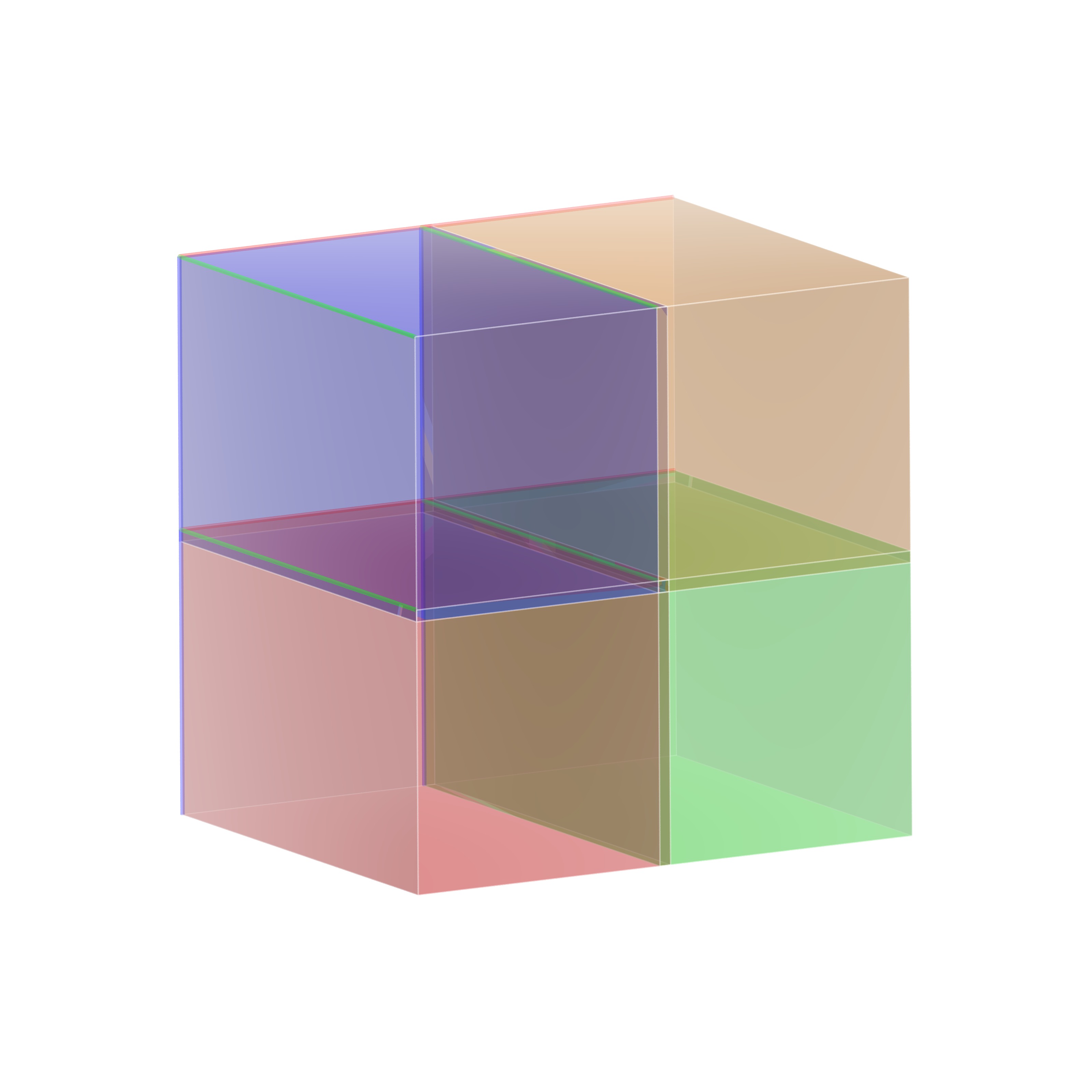
Here we visualize an example set of gist sub-volumes generated by this command:

CLICK HERE TO GO BACK TO SECTION 3 RETURN TO INDEX

(Note: These tutorials are meant to provide illustrative examples of how to use the AMBER software suite to carry out simulations that can be run on a simple workstation in a reasonable period of time. They do not necessarily provide the optimal choice of parameters or methods for the particular application area.)
Copyright Ross Walker 2015