


Simple Simulation of Alanine Dipeptide*
*formerly Tutorial B0By Benjamin D. Madej & Ross Walker
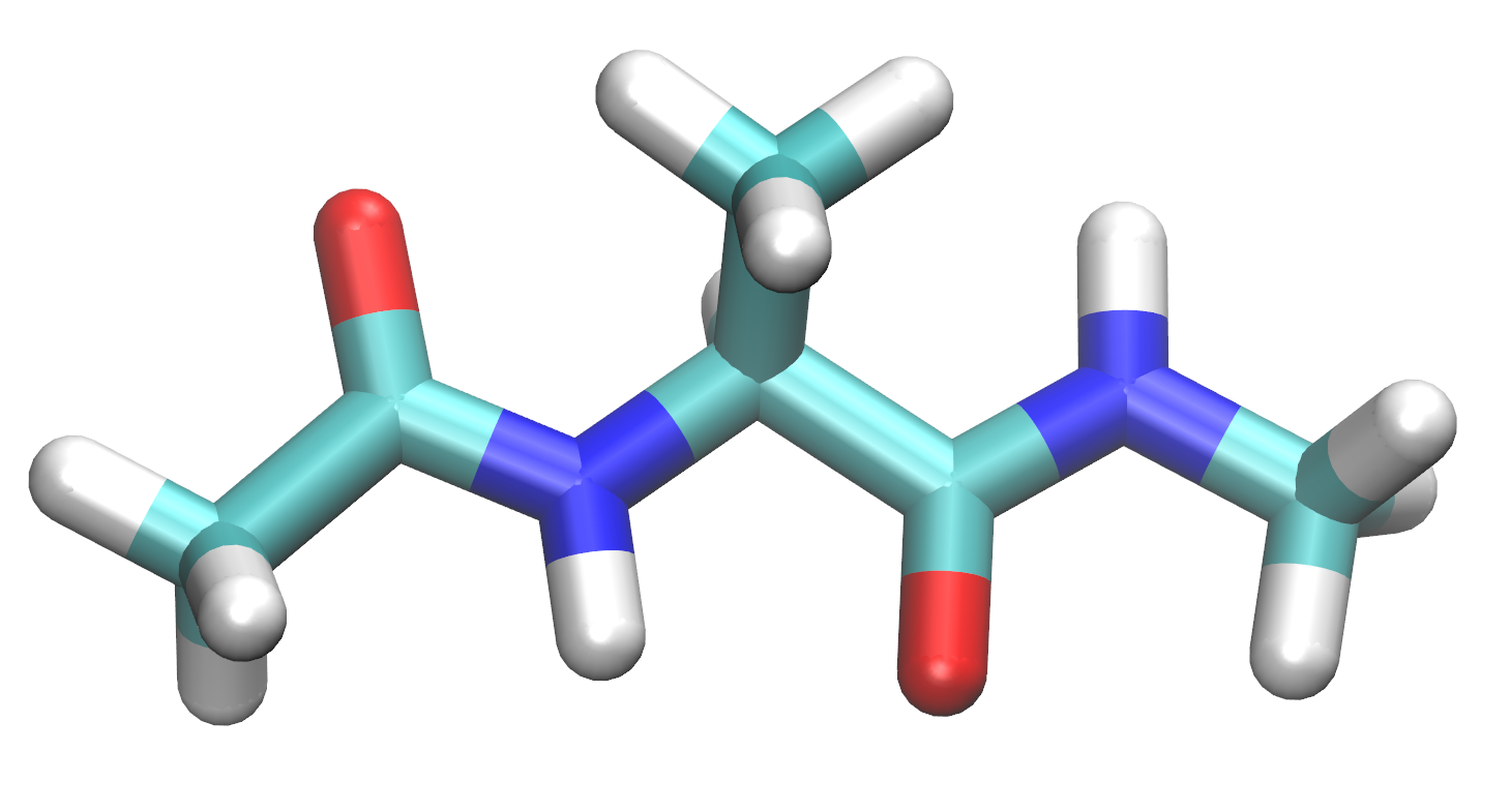
TABLE OF CONTENTS
Learning Outcomes
Introduction
Prepare topology and
coordinate files
Load a
protein force field
Build alanine dipeptide
Solvate alanine
dipeptide
Save the
Amber parm7 and rst7 input files
Prepare Amber MD pmemd and sander input
files
Minimization input
Heating input
Production input
Run Amber MD sander
Run minimization
Run heating MD
Run production MD
Visualize the results
Analyze the MD results
Production MD
system properties
Use cpptraj to analyze the
RMSD
Conclusion
Learning Outcomes
After completing this tutorial you will be able to:
- navigate the command line interface through terminal and tleap to prepare topology and coordinate files
- understand the basics of forcefields and be able to load the FF19SB forcefield to be able to work with the alanine dipeptide
- set up an explicit water simulation in tleap
- perform basic equilibration
- perform production run simulations at a given temperature
- Visualize the results of production MD in VMD or Chimera-X
- Use xmgrace to plot MD thermodynamic data such as temperature, density, and energy
- Use cpptraj to calculate the root mean square displacement (RMSD) of the trajectory relative to the initial structure
Introduction
This tutorial is designed to provide an introduction to molecular dynamics simulations with Amber. It is designed around AMBER v20 and for new users who want to learn about how to run molecular dynamics simulations with Amber.It does however assume that you have a machine with Amber v20, VMD and xmgrace correctly installed.
AMBER stands for Assisted Model Building and Energy Refinement. It refers not only to the molecular dynamics programs, but also a set of force fields that describe the potential energy function and parameters of the interactions of biomolecules.
In order to run a Molecular Dynamics simulation in Amber, each molecule's interactions are described by a molecular force field. The force field has specific parameters defined for each molecule.
sander is the basic MD engine of Amber. pmemd is the high performance implementation of the MD engine that contains a subset of features of sander. pmemd can also be run with acceleration from graphics processing units (GPU) through pmemd.cuda or the MPI parallel version pmemd.mpi. For a tutorial on specifically running pmemd.cuda see Tutorial 3.2 Running MD with pmemd.
In order to run an MD simulation with sander or pmemd, three key files are needed:
- parm7 - The file that describes the parameter and topology of the molecules in the system
- rst7 - The file that describes the initial molecular coordinates of the system
- mdin - The file that describes the settings for the Amber MD engine
Prepare topology and coordinate files
Amber MD is software that is entirely based on a Command Line Interface (CLI) on a computer running Unix. To learn more about Unix commands and vi text editor, please see the tutorials under Tools. For help learning the command line in Unix, see:- 10.1.1 Introduction to Unix tutorial
- Codecademy command line tutorial
- Ryan's Linux tutorial
- Vi editor
Note that the "$" is the command line prompt in the terminal. You'll need a new directory for the files and folders created in this tutorial.
2. Make a new directory for this tutorial with the mkdir command called Tutorial.
$ mkdir TutorialAt this point, you'll want to move into your Tutorial directory so that you can save all of your working files there.
3. Use the cd command to change to different directory.
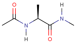
$ cd TutorialFor this tutorial, you will build the following molecule in the preparatory program called tLEaP for simulation in AMBER.
$ ls
4. Start tLEaP now with the tleap command.
> tleap
-I: Adding /home/packages/amber20/dat/leap/prep to search path.
-I: Adding /home/packages/amber20/dat/leap/lib to search path.
-I: Adding /home/packages/amber20/dat/leap/parm to search path.
-I: Adding /home/packages/amber20/dat/leap/cmd to search path.

Welcome to LEaP!
(no leaprc in search path)
>
Load a protein force field
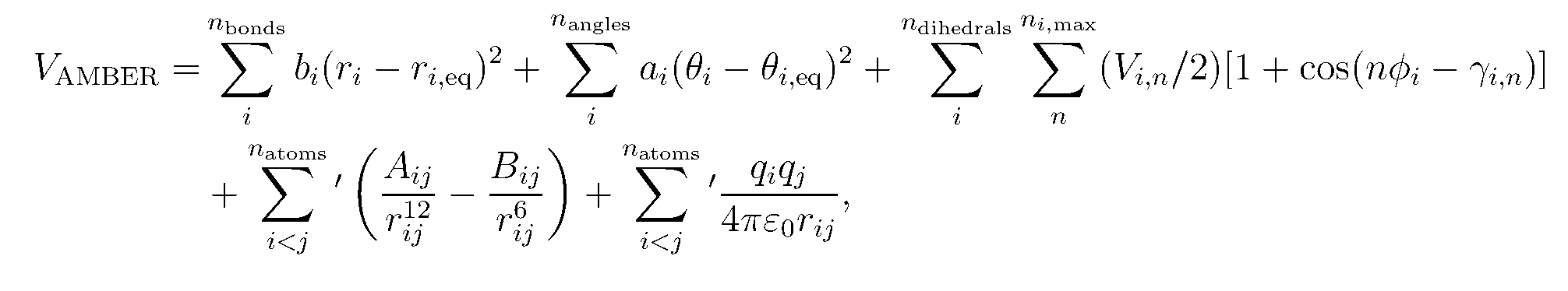
A force field is the Hamiltonian (potential energy function) and the related parameters that describe the intra- and intermolecular interactions between the molecules in the system. In MD, the Hamiltonian is integrated to describe the forces and velocities of the molecules (See Allen and Tildesley).The basic form of the Amber force field is:
5. source (load) the FF19SB force field now.
> source leaprc.protein.ff19SB
----- Source: /home/packages/amber20/dat/leap/cmd/leaprc.protein.ff19SB
----- Source of /home/packages/amber20/dat/leap/cmd/leaprc.protein.ff19SB done
Log file: ./leap.log
Loading parameters: /home/packages/amber20/dat/leap/parm/parm19.dat
Reading title:
PARM99 + frcmod.ff99SB + frcmod.parmbsc0 + OL3 for RNA + ff19SB
Loading parameters: /home/packages/amber20/dat/leap/parm/frcmod.ff19SB
Reading force field modification type file (frcmod)
Reading title:
ff19SB AA-specific backbone CMAPs for protein 07/25/2019
Loading library: /home/packages/amber20/dat/leap/lib/amino19.lib
Loading library: /home/packages/amber20/dat/leap/lib/aminoct12.lib
Loading library: /home/packages/amber20/dat/leap/lib/aminont12.lib
>
Build alanine dipeptide
We can build an alanine dipeptide as an alanine amino acid capped with an acetyl group on the N-terminus and N-methylamide on the C-terminus. After we loaded the force field ff19SB, tLEaP now has these "units" available to build into a molecule. The sequence command will create a new unit from the available units and connect them together.6. Use sequence to create a new unit called diala out of the ACE, ALA, and NME units.
Note that the ">" indicates the command line in tLEaP.
> diala = sequence { ACE ALA NME }
Now you have a single alanine dipeptide molecule stored in the unit diala.
Solvate alanine dipeptide
The next step to prepare this alanine dipeptide system is to solvate the molecule with explicit water molecules. There are many water models available for MD simulations. In this simulation we will add OPC water molecules2 to the system. The ff19SB force field gives the best performance with the OPC water model and is strongly recommended (see page 36 of the Amber 2020 Manual). To learn more about the OPC water model, please look at section 3.5.1 on pages 53 and 54 of the Amber 2020 Manual.In this type of simulation, the system has periodic boundary conditions, meaning that molecules that exit one side of the system will wrap to the other side of the system. It is important that the periodic box is large enough, i.e. there is enough water surrounding alanine dipeptide, so that the alanine dipeptide molecule does not interact with its periodic images.
7. Solvate the system with the solvateoct command.
> source leaprc.water.opc
> solvateoct diala OPCBOX  10.0
OPCBOX specifies the type of specifies the type of water box to solvate the solute (diala). The 10.0 indicates that the molecule should have a buffer of at least 10 Angstroms between alanine dipeptide and the periodic box wall.
Save the Amber parm7 and rst7 input files
Now we will save the parm7 and rst7 files to the current working directory. The parm7 topology file defines which atoms are bonded to each other and the rst7 coordinate file defines where each atom is located on a 3-dimensional coordinate plane. The unit diala now contains the alanine dipeptide molecule, water molecules, and the periodic box information necessary for simulation. The parameters will be assigned from the ff19SB force field.8. To save the parm7 and rst7 file use the saveamberparm command.
> saveamberparm diala parm7 rst7Warning:
Checking Unit.
Building topology.
Building atom parameters.
Building bond parameters.
Building angle parameters.
Building proper torsion parameters.
Building improper torsion parameters.
total 4 improper torsions applied
Building H-Bond parameters.
Incorporating Non-Bonded adjustments.
Not Marking per-residue atom chain types.
Marking per-residue atom chain types.
(no restraints)
Pay close attention to the output of this command for any warnings or errors that your parm7 and rst7 file did not build correctly.
Amber parameter/topology and coordinate files
The alanine dipeptide parm7 and input files are available here:parm7
rst7
Quit tLEaP
9. To quit tLEaP use quit.> quit
Prepare Amber MD pmemd and sander input files
The last components needed are the input files that define the program settings for each MD run. For this system, we will perform an energy minimization on the system, then slowly heat the system, and then do production MD at the desired temperature and pressure. Sander will be used for minimization and heating and pmemd will be used for the actual production run. To learn more about sander and pmemd, please refer to the Amber 2020 Manual.- Minimization
- Heating with constant volume and temperature (NVT) for 20 ps from 0 K to 300 K
- Production MD with constant pressure and temperature (NPT) at 300 K and 1 atm for 60 ps
To control all these settings, we will write a simple input file in a text editor. Unix has many text editors available, but we will use one of two simple text editors included on your computer.
10. Open the gedit Text Editor or the VI Text Editor on your Linux computer.
Minimization input
11. Create the file 01_Min.in that includes the following settings for minimization:MinimizeThe settings can be summarized as follows:
&cntrl
imin=1,
ntx=1,
irest=0,
maxcyc=2000,
ncyc=1000,
ntpr=100,
ntwx=0,
cut=8.0,
/
| imin=1 |
Choose a minimization run |
| ntx=1 |
Read coordinates but not velocities
from ASCII formatted rst7
coordinate file |
| irest=0 |
Do not restart simulation. (not
applicable to minimization) |
| maxcyc=2000 |
Maximum minimization cycles |
| ncyc=1000 |
The steepest descent algorithm for
the first 0-ncyc cycles,
then switches the conjugate gradient algorithm for ncyc-maxcyc
cycles |
| ntpr=100 |
Print to the Amber mdout
output file every ntpr
cycles |
| ntwx=0 |
No Amber mdcrd
trajectory file written (not applicable to minimization) |
| cut=8.0 |
Nonbonded cutoff distance in
Angstroms (for PME, limit of the direct space sum - do NOT reduce
this below 8.0. Higher numbers give slightly better accuracy but
at vastly increased computational cost.) |
For more information on minimization, please take a look at the General minimization and dynamics parameters section on page 340 of the Amber 2020 Manual.
Heating input
12. Create the file 02_Heat.in that includes the following settings for heating:HeatThe settings can be summarized as follows:
&cntrl
imin=0,
ntx=1,
irest=0,
nstlim=10000,
dt=0.002,
ntf=2,
ntc=2,
tempi=0.0,
temp0=300.0,
ntpr=100,
ntwx=100,
cut=8.0,
ntb=1,
ntp=0,
ntt=3,
gamma_ln=2.0,
nmropt=1,
ig=-1,
/
&wt type='TEMP0', istep1=0, istep2=9000, value1=0.0, value2=300.0 /
&wt type='TEMP0', istep1=9001, istep2=10000, value1=300.0, value2=300.0 /
&wt type='END' /
| imin=0 |
Choose a molecular dynamics (MD)
run [no minimization] |
| nstlim=10000 |
Number of MD steps in run (nstlim *
dt = run length in ps) |
| dt=0.002 |
Time step in picoseconds (ps). The
time length of each MD step |
| ntf=2 |
Setting to not calculate force for
SHAKE constrained bonds |
| ntc=2 |
Enable SHAKE to constrain all bonds
involving hydrogen |
| tempi=0.0 |
Initial thermostat temperature in K
(see NMROPT section) |
| temp0=300.0 |
Final thermostat temperature in K
(see NMROPT section) |
| ntwx=1000 |
Write Amber trajectory file mdcrd
every ntwx steps |
| ntb=1 |
Periodic boundaries for constant
volume |
| ntp=0 |
No pressure control |
| ntt=3 |
Temperature control with Langevin
thermostat |
| gamma_ln=2.0 |
Langevin thermostat collision
frequency |
| nmropt=1 |
NMR restraints and weight changes
read (see NMROPT section) |
| ig=-1 |
Randomize the seed for the
pseudo-random number generator [always a good idea unless you are
debugging a simulation problem] |
For more information on heating, please take a look at the Temperature regulation subsection on page 345 of the Amber 2020 Manual.
Thermostat temperature via NMROPT
The final three lines allow the thermostat to change its target temperature throughout the simulation. For the first 9000 steps, the temperature will increase from 0 K to 300 K. For steps 9001 to 10000, the temperature will remain at 300 K.Production input
Warning:By itself, this input file is not intended for general MD simulations.
NTPR and NTWX are set very low so that it is possible to analyze this short simulation. Using these settings for longer MD simulations will create very large output and trajectory files and will be slower than regular MD. For real production MD, you'll need to increase NTPR and NTWX.
The production time of this simulation will be 10 ns. Using a time step (dt) of 0.002 ps, a nstlim value of 5000000 will give us this simulation time.
13. Create the file 03_Prod.in with the settings for production MD:
ProductionThe settings for production can be summarized as follows:
&cntrl
imin=0,
ntx=5,
irest=1,
nstlim=5000000,
dt=0.002,
ntf=2,
ntc=2,
temp0=300.0,
ntpr=100,
ntwx=100,
cut=8.0,
ntb=2,
ntp=1,
ntt=3,
barostat=1,
gamma_ln=2.0,
ig=-1,
/
| ntx=5 |
Read coordinates and velocities
from unformatted rst7
coordinate file |
| irest=1 |
Restart previous MD run [This means
velocities are expected in the rst7 file and will be used to
provide initial atom velocities] |
| temp0=300.0 |
Thermostat temperature. Run at 300K |
| ntb=2 |
Use periodic boundary conditions
with constant pressure |
| barostat=1 |
Use the Berendsen barostat for
constant pressure simulation |
For more information on pressure control, please take a look at the Pressure regulation subsection on page 347 of the Amber 2020 Manual.
Input files
The pmemd input files are available here:01_Min.in
02_Heat.in
03_Prod.in
Run Amber MD pmemd
Now that we have all the ingredients: the parameter and topology file parm7, the coordinate file rst7, and the input files 01_Min.in, 02_Heat.in, 03_Prod.in, we are ready to run the actual minimization, heating, and production MD.To do this, we will use the program pmemd which is run from the command line. On the command line, we can specify several more options and choose which files are to be used for input.
14. First, from the terminal, you will need to change directories to the Tutorial directory with all of your input files. "~" is a shortcut to your home directory where you created a Tutorial directory.
$ cd ~/Tutorial
Run minimization
15. Run the minimization of alanine dipeptide with sander.$ $AMBERHOME/bin/sander -O -i 01_Min.in -o 01_Min.out -p parm7 -c rst7 -r 01_Min.ncrst \ -inf 01_Min.mdinfosander uses a consistent syntax for each step of MD simulation. Here is a summary of the command line options of sander:
| -O |
Overwrite the output files if they
already exist |
| -i 01_Min.in |
Choose input file (default mdin) |
| -o 01_Min.out |
Write output file (default mdout) |
| -p parm7 |
Choose parameter and topology file
parm7 |
| -c rst7 |
Choose coordinate file rst7 |
| -r 01_Min.ncrst |
Write output restart file with
coordinates and velocities (default restrt) |
| -inf 01_Min.mdinfo |
Write MD info file with simulation
status (default mdinfo) |
To learn more about syntax when using sander, please look at Section 19.2 of the Amber 2020 Manual.
sander should complete the minimization in a moderate amount of time (~ 30 seconds) depending on your computer specifications.
After sander completes, there should be an output file 01_Min.out, a restart file 01_Min.ncrst, and a MD info file 01_Min.mdinfo. You will use the restart file 01_Min.ncrst for the heating of the system.
Minimization output files
The minimization output files are available here:01_Min.out
01_Min.ncrst
16. Using gedit, VI, or the Unix commands less or more, look at the output file 01_Min.out.
less 01_Min.outor
more 01_Min.outIn the 01_Min.out file, you will find the details of your minimization. You should be able to see the system energy ENERGY decrease throughout the minimization.
Run heating MD
Now, using the restart file from the initial minimization, we will heat the system.17. Run the heating of alanine dipeptide with sander.
$ $AMBERHOME/bin/sander -O -i 02_Heat.in -o 02_Heat.out -p parm7 -c 01_Min.ncrst \
-r 02_Heat.ncrst -x 02_Heat.nc -inf 02_Heat.mdinfo
Here is a summary of the command line options for sander:
| -c 01_Min.ncrst |
Now for the input coordinates we
choose the restart file from minimization |
| -x 02_Heat.nc |
Output trajectory file for MD
simulation (default nc) |
sander should complete the heating in a moderate amount of time (~ 2.5 mins) depending on your computer specifications.
Heating output files
The heating output files are available here. Some files are compressed and need to be unzipped.02_Heat.out
02_Heat.ncrst
02_Heat.nc
18. Open the output file 02_Heat.out to view the system output.
In the 02_Heat.out file you will find the output from the heating MD. You should be able to see system information including timestep energies, and temperature. For example on the 1000 time step:
NSTEP = 1000 TIME(PS) = 2.000 TEMP(K) = 30.80 PRESS = 0.0Some of the important values include:
Etot = -9636.4025 EKtot = 130.0070 EPtot = -9766.4095
BOND = 0.5896 ANGLE = 1.6788 DIHED = 2.6834
1-4 NB = 2.8404 1-4 EEL = 45.1563 VDWAALS = 1584.9308
EELEC = -11403.7559 EHBOND = 0.0000 RESTRAINT = 0.0000
CMAP = -0.5328
Ewald error estimate: 0.4716E-03
------------------------------------------------------------------------------
NMR restraints: Bond = 0.000 Angle = 0.000 Torsion = 0.000
===============================================================================
| NSTEP |
The time step that the MD
simulation is at |
| TIME |
The total time of the simulation
(including restarts) |
| TEMP |
System temperature |
| PRESS |
System pressure |
| Etot |
Total energy of the system |
| EKtot |
Total kinetic energy of the system |
| EPtot |
Total potential energy of the
system |
Note that the pressure is 0.0 because the barostat (pressure control) is not being used in the heating.
Run production MD
Now that minimization and heating are complete. We move on to the actual production MD.19. Run the production MD of alanine dipeptide with pmemd.
$ $AMBERHOME/bin/pmemd -O -i 03_Prod.in -o 03_Prod.out -p parm7 -c 02_Heat.ncrst \
-r 03_Prod.ncrst -x 03_Prod.nc -inf 03_Prod.info &
Note: With the "&" at the end of the command, sander now runs in the background
Now pmemd is running in the background.
But we'd like to monitor the status of the production MD. So we will monitor the pmemd output file to check the status of the run. The Linux program tail will print the end of the output file.
20. To monitor the status of this job use the program tail to print the output file to the terminal.
$ tail -f 03_Prod.outThis prints the output file as pmemd is running. It's useful to keep track of the job. You can also monitor the mdinfo file (cat 03_Prod.info) which provides detailed performance data as well as estimated time to completion.
21. To exit tail, quit the program by pressing <CTRL-C>.
Complete the MD simulation
Let the MD simulation run. It should take a while to complete the simulation [~ 13 hours].Production output
The production MD output file is available here:03_Prod.out
Once the production run is complete open the output file to check that the simulation completed normally.
22. Open the output file 03_Prod.out with gedit or VI to view the output of the MD simulation.
Visualize the results
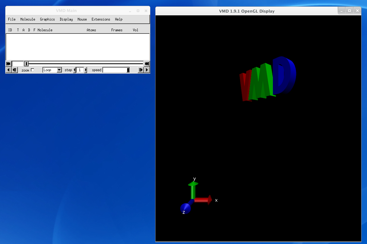
You've now run an MD simulation. In order to visualize the results, we will now use a program called VMD (Visual Molecular Dynamics). This is a molecular graphics program that can render molecular structures in 3D. VMD not only loads Protein Database (PDB) structure files, but also MD trajectories from many programs. [A more in-depth tutorial on VMD is available as an optional hands-on session listed at the bottom of the workshop program page].23. To start VMD, open a terminal, change directory to your tutorial files in the Tutorial directory, and run vmd. Remember ~/Tutorial is a shortcut to your Tutorial directory.
$ cd ~/TutorialVMD should look like this:
$ vmd
VMD is a very useful tool to visualize protein, nucleic acid, and other biomolecular atomic structures. One of the most common formats is the PDB biomolecular structure format. To load a PDB, got to File -> New Molecule.... Then load files for a New Molecule and choose the PDB file. VMD should determine the file type Automatically.
However, we would like to visualize the alanine dipeptide trajectory. Now we will load our MD trajectory to look at the dynamics of alanine dipeptide.
24. Create a new molecule with File -> New Molecule...
25. Load files for New Molecule. Then choose the Amber parameter and topology file parm7. Set the file type to AMBER7 Parm. Click Load.
26. Load files for 0: parm7. Then choose the Amber trajectory file 03_Prod.nc. Set the file type to NetCDF (AMBER, MMTK). Click Load.
VMD now loads your trajectory to be visualized. The main VMD window can be used to control playback. For more tutorials using VMD, see the tutorials under VMD and Tools.
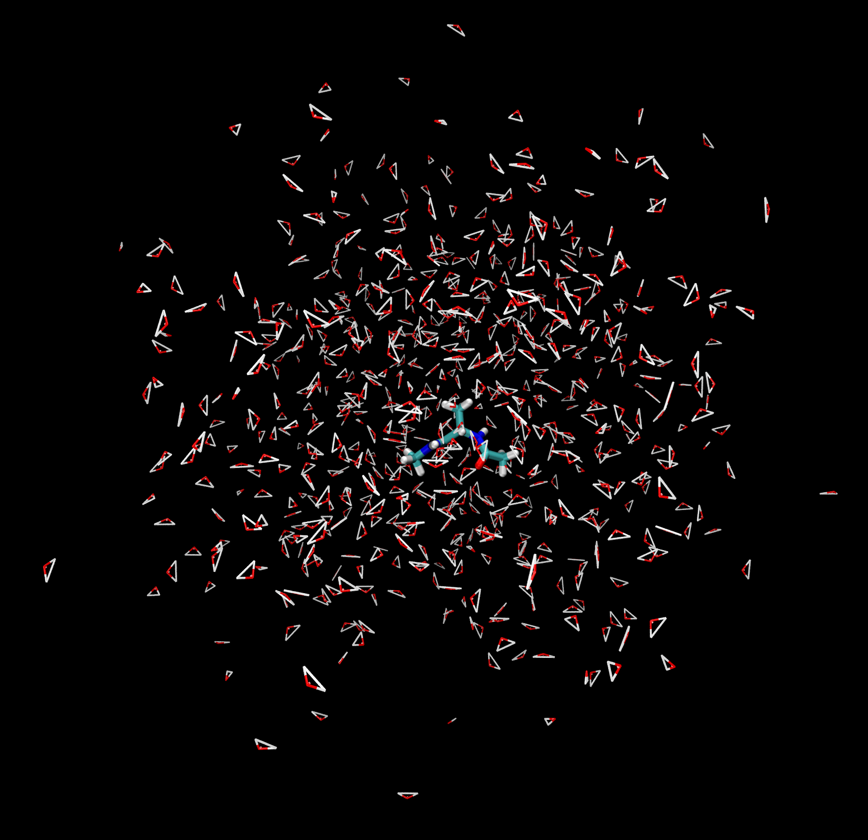
You should be able to see the alanine dipeptide molecule as well as the many water molecules in the display. You can rotate, zoom and pan the molecules around the display with the mouse.
Many different visualization options can be changed in the Graphics -> Representations window.
Your visualization can be restricted to the alanine dipeptide as well.
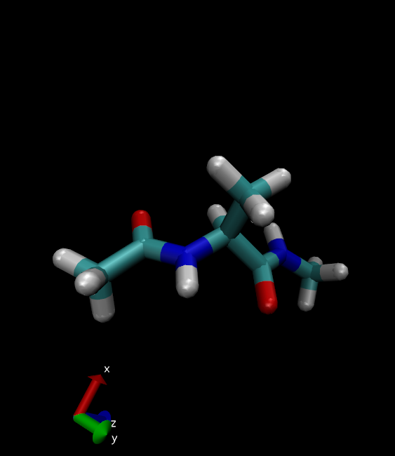
27. Change the Selected Atoms to all not water.
You can change the drawing method for the molecule to a more interesting model.
28. Change the Drawing Method to Licorice.
Alanine dipeptide will look something like this:
More VMD
VMD has a lot of functions that can be used to analyze and study a MD trajectory. For example it is possible to align molecules, measure root mean squared deviations (RMSD), save structures from a trajectory, and measure physical system parameters throughout a trajectory. It's also possible to render a movie of a trajectory.However, these functions are beyond the scope of this introductory section. For more details please refer to the official VMD Tutorials.
Analyze the MD results
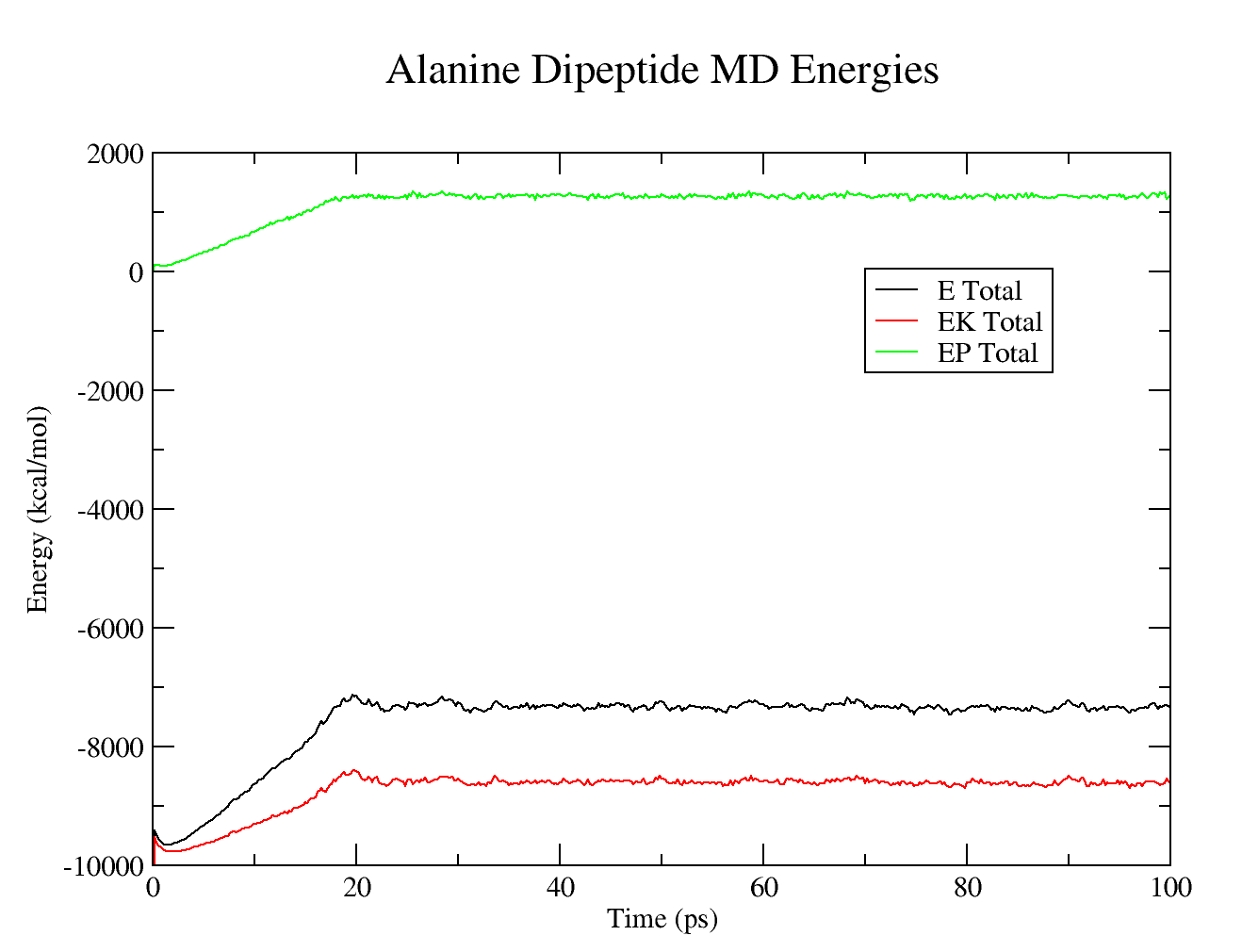
Amber includes a suite of tools to examine and analyze MD trajectories. In this tutorial, we will do a simple analysis with a script to analyze thermodynamic parameters and an introductory analysis with cpptraj. More cpptraj tutorials can be found under the Trajectory Analysis Tutorials.The results will then be plotted with XMGrace but could also be done with pyplot (see Tools links. The analysis will primarily be done from the command line in the terminal.
29. Open a terminal and change directory to your tutorial files.
$ cd ~/Tutorial30. Make an Analysis directory and change to that directory.
$ mkdir AnalysisNow we will use an analysis script process_mdout.perl to analyze the MD output files. This script will extract the energies, temperature, pressure, density, and volume from the MD output files and save them to individual data files.
$ cd Analysis
31. Process the MD output files with process_mdout.perl
$ $AMBERHOME/bin/process_mdout.perl ../02_Heat.out ../03_Prod.outIt is now quite simple to plot the data saved in the output files.
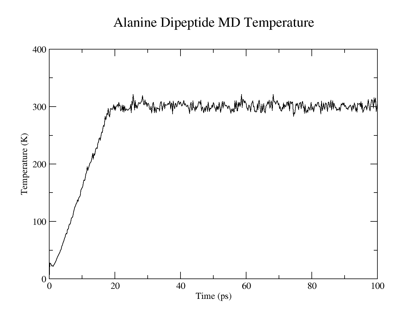
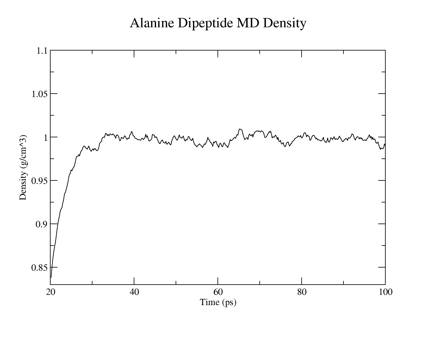
We will use a convenient, simple plotting program called xmgrace to automatically generate plots for the following MD simulation properties throughout the simulation. We use this for our convenvience, but you can use any plotting program of your choice.
- MD simulation temperature
- MD simulation density
- MD simulation total, potential, and kinetic energies.
32. Use gedit or VI to edit the summary.DENSITY file to remove the empty data points (up to 20 ps).
33. Plot these properties through the simulation using the following commands.
$ xmgrace summary.TEMP
$ xmgrace summary.DENSITY
$ xmgrace summary.ETOT summary.EPTOT summary.EKTOT
Analysis data files
The analysis data files are available here:summary.TEMP
summary.DENSITY
summary.ETOT
summary.EPTOT
summary.EKTOT
Production MD system properties
Warning:We should run this simulation much longer so that the density has equilibrated and the simulation converges. However, in the interest of time for this tutorial, the production MD simulation time has been set very low so that it possible to analyze the results.
The resulting plots should look similar to these:
Use cpptraj to analyze the RMSD
The root mean squared deviation (RMSD) value is a measurement of how similar a structure's internal atomic coordinates are relative to some reference molecule coordinates. For this example, we will measure how the internal atomic coordinates change relative to the minimized structure. Specifically, we will analyze the alanine atoms (residue 2).To do this analysis, we will use cpptraj, a fairly comprehensive analysis program for processing MD trajectories. This program runs simple user-written scripts that choose what trajectories to load, what analysis to run, and what processed trajectories or structure to save.
First, we will need to write a simple cpptraj script to do this analysis.
34. Use gedit or VI to create a cpptraj script called rmsd.cpptraj.
trajin 02_Heat.ncThis is a brief summary of the cpptraj script:
trajin 03_Prod.nc
reference 01_Min.ncrst
autoimage
rms reference mass out 02_03.rms time 2.0 :2
| trajin 02_Heat.nc |
Load the trajectory 02_Heat.nc |
| reference 01_Min.ncrst |
Define the structure 01_Min.ncrst as
the reference structure |
| center :1-3 mass origin |
Center the residues 1-3 by mass to
the system origin |
| image origin center |
Image the atoms to the origin using
the center of mass of the molecule |
| rms reference mass out 02_03.rms
time 2.0 :2 |
Calculate the mass weighted RMSD
using the reference and output to 02_03.rms |
To learn more about calculating rmsd's with cpptraj please look at section 32.21.3 and section 32.10.4 on page 637 of the Amber 2020 Manual.
Cpptraj input script file
The cpptraj input script file is available here:rmsd.cpptraj
Run cpptraj
To actually run cpptraj, we must run it again from the terminal in the directory where the parm7, nc, and reference ncrst file is located.35. Using the terminal, change directory to your Tutorial folder, and run cpptraj. A parm7 file and cpptraj script must be specified.
$ cd ~/TutorialNow our RMSD data is stored in the file 02_03.rms. We can simply plot this file with xmgrace.
$ $AMBERHOME/bin/cpptraj -p parm7 -i rmsd.cpptraj &> cpptraj.log
36. Plot the RMSD with xmgrace.
If you need to download xmgrace or if you want to use pyplot instead, see resources under Plotting tutorials.
$ xmgrace 02_03.rms
Cpptraj output files
The cpptraj output files are available here:02_03.rms
cpptraj.log
Alanine dipeptide MD RMSD relative to minimized initial structure

Conclusion
Congratulations. You've now run your first complete MD simulation and successfully analyzed the results. This is a fairly simple example of the workflow for setting up, running, and analyzing your own MD simulation. If you want to learn more you are encouraged to complete the additional tutorials on the AMBER website.Copyright Ross Walker & Ben Madej, 2015
Updated for Amber 15 by Aditi Munshi and Ross Walker
Updated for Amber 18 by Sifath Mannan, Michael Barton and Tyler Luchko
Last updated for Amber 20 and tLEaP by Jan Ziembicki and Maria Nagan