Running MD with pmemd

Learning Objectives

• Be able to run pmemd on GPUs
  
• Understand the components of a basic molecular dynamics production run input file.
  
• nstlim
  
• ntpr, ntwx and ntwr
  
• dt
  
• ntt
  
• ntp
  
• Running the MD Production Run
  

Introduction

This tutorial will introduce you to running a molecular dynamics(MD) simulation under production run conditions using pmemd. It will use the protein system prepared in Tutorial 1.4: Building Protein Systems in Explicit Solvent to run the simulation. Note that this tutorial only covers the production run, and does not go over minimization, heating, or equilibration.

Running on GPUs with pmemd

Particle Mesh Ewald Molecular Dynamics (PMEMD) is the primary engine for running MD simulations with AMBER. Sander can still employed to run MD production runs on CPUs but it will be much slower. The pmemd.CUDA executable provides the ability to use NVIDIA GPUs to greatly decrease the time it takes to run explicit and implicit solvent simulations. Previously, sander was the primary engine, but pmemd has several performance improvements for using GPUs in serial and in parallel. The functionality of pmemd supports Particle Mesh Ewald simualtions, Generalized Born simulations, Isotropic Periodic Sums, ALPB solvent, and gas phase simulations using AMBER and CHARMM forcefields. As such, we recommend using pmemd whenever possible. Note that pmemd is not a complete implementation of sander. See the pmemd section of the Amber Reference Manual for more information.

Input File

Once a system is built equilibration follows, in which the positional restraints that were imposed on the system for minimization and heating are slowly removed and the system is heated. There are usually no positional restraints imposed on the system in the production run, and for this reason it is sometimes called "unrestrained MD". The production run is the only focus of any analysis.

To run a production run, there are three required files. These are:

1. A topology file generated by LEaP ( RAMP1.prmtop)
2. A coordinate file of the equilibrated system ( RAMP1_equil.rst7)
3. A md.in input file (below)

The md.in input file specifies the conditions of the production run.

1. Download all 3 files needed and place them in the same directory

md.in

Explicit solvent molecular dynamics constant pressure 50 ns MD
 &cntrl
   imin=0, irest=1, ntx=5, 
   ntpr=500000, ntwx=500000, ntwr=500000, nstlim=25000000, 
   dt=0.002, ntt=3, tempi=300, 
   temp0=300, gamma_ln=1.0, ig=-1, 
   ntp=1, ntc=2, ntf=2, cut=9, 
   ntb=2, iwrap=1, ioutfm=1, 
/ 

These settings are appropriate for a short simulation (50 ns) of a protein system in a truncated octahedral box solvated in explicit water, but you may need to change some aspects of it for your own system. In this tutorial, we will only be discussing the most important flags. See the Amber Reference Manual for information on the other flags.

nstlim

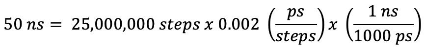
The nstlim flag controls how long your simulation is by telling the program how many steps of MD to run. Multiplication of the time step by the number of steps will give you the length of the simulation in ps. Here, 25,000,000 steps translates to 50 ns of real-time simulation. If you want to run for a different amount of time, you will have to change the value of nstlim.



ntpr, ntwx and ntwr

The ntpr, ntwx, and ntwr variables control how often a frame of the simulation is saved. Here, ntpr=500,000 translates to saving every 500,000 steps or 1 ns in the md.out file. The ntwx namelist parameter refers to how often the frame will be saved to the restart file. The ntwr namelist parameter writes to the trajectory file (RAMP1_md.nc). You may need to adjust this parameter to write out more often if you are looking at finer changes.

dt

This variable is the time step in picoseconds (1 ps = 10^-12 s). The time step is basically the time unit of MD simulations. Here, it is 0.002 ps, which is 2.0 fs.

As for choosing what the time step of your simulation should be, it depends on the temperature and if the SHAKE algorithm is used. Here, we do use the SHAKE algorithm (ntb=2, btc=2, and ntf=2), so the maximum time step should be 0.002 (0.001 if the SHAKE algorithm is not used). For temperatures above 300 K, the time step should be reduced. This is because the increased velocity will lead to longer distances travelled in between force evaluations, which could cause the system to blow up.

ntt

This variable defines which thermostat is used. Here, we use the Langevin thermostat (ntt=3). Langevin dynamics are susceptible to "synchronization" artifacts, so the ig variable needs to be specifically set to counter this. It is recommended that ig be set to -1 (the default) for ntt=3. When ig=-1, the random seed is based on the current time and date, so it will be different for each run.

ntp

This is the variable that controls pressure dynamics. Because we want to run our simulation under conditions of constant pressure, it should be set equal to 1 (which corresponds to MD with isotropic position scaling). If the system is in an orthogonal box (meaning all angles are 90 degrees), then it should be set to 2. Because the box for this simulation is a truncated octahedron, we should set it equal to 1. The Berendsen barostat is used by default.

Running the MD Production Run

Now that we have all of the necessary files for running an MD simulation, we can run it. Running MD on a GPU requires a jobfile script.

2. Make the jobfile script using the text editor vi

vi jobfile_production.sh

If you are unfamiliar with the use of vi, see this tutorial.

a. Type in the jobfile_production.sh contents

#! /bin/bash -f

export CUDA_VISIBLE_DEVICES=0

$AMBERHOME/bin/pmemd.cuda -O -i md.mdin -p RAMP1.prmtop -c RAMP1_eq7.rst7\
 -ref RAMP1_eq7.rst7 -o RAMP1_md.mdout -r RAMP1_md.rst7 -x RAMP1_md.nc

You can also download the Jobfile here. Below are flags used in jobfile_production.sh.

-O   Overwrite output files
-i   input file (md.in, which can be found above)
-p   topology file (RAMP1.prmtop)
-c   the starting coordinate file (RAMP1_equil.rst7)
-ref reference coordinates; use the same as the starting coordinates
-o   output file (RAMP1_md.out)
-r   restart file (last set of xyz coordinates from the simulation)
-x   file with trajectory (RAMP1_md.nc) 

b. Edit the jobfile indicating the GPU to run the job.

The export CUDA_VISIBLE_DEVICES=0 line tells the computer to run on the GPU designated 0. You will likely have to change this to run on a GPU that is open on your computer. You can see which GPUs are open with this command:

nvidia-smi

Which will output this information.

+-----------------------------------------------------------------------------+
| NVIDIA-SMI 440.33.01    Driver Version: 440.33.01    CUDA Version: 10.2     |
|-------------------------------+----------------------+----------------------+
| GPU  Name        Persistence-M| Bus-Id        Disp.A | Volatile Uncorr. ECC |
| Fan  Temp  Perf  Pwr:Usage/Cap|         Memory-Usage | GPU-Util  Compute M. |
|===============================+======================+======================|
|   0  GeForce RTX 208...  On   | 00000000:02:00.0 Off |                  N/A |
| 84%   88C    P8   112W / 250W |      0MiB /  7979MiB |      97%     Default |
+-------------------------------+----------------------+----------------------+
|   1  GeForce RTX 208...  On   | 00000000:04:00.0 Off |                  N/A |
| 81%   86C    P8    96W / 250W |      0MiB /  7982MiB |      96%     Default |
+-------------------------------+----------------------+----------------------+
|   2  GeForce RTX 208...  On   | 00000000:05:00.0 Off |                  N/A |
| 77%   84C    P8   122W / 250W |      0MiB /  7982MiB |      96%     Default |
+-------------------------------+----------------------+----------------------+
|   3  GeForce RTX 208...  On   | 00000000:06:00.0 Off |                  N/A |
| 24%   26C    P8     3W / 250W |      0MiB /  7982MiB |      0%      Default |
+-------------------------------+----------------------+----------------------+
                                                                               

On this computer, there are four GPUs (0, 1, 2, and 3; listed on the left). Their respective availability is shown on the right. Here, GPUs 0, 1, and 2 are unavailable, but GPU 3 is open. So, we want to tell the computer to run our job on GPU 3 by changing the second line to reflect this:

export CUDA_VISIBLE_DEVICES=3

This will make the job run on the open GPU 3.

The last line is what runs the simulation using pmemd.cuda (the GPU version).

3. Once you have written the script, save it and run it in the command line by typing:

 ./Jobfile_production.sh &

The & makes the job run in the background, meaning you can continue to use the command line.

4. Verify that your job is running by using the nvidia-smi command again.

nvidia-smi

You should see that the percentage of the GPU you specified increased to a percentage near 100%. You can also see information on your job by using the "top" command:

top

This will show you the PID (first column), who is running the job (second column), and what kind of job it is (last column), which should be pmemd.cuda for you. The "top" screen will be automatically updated in real time. To exit back to the command line, type the "q" key on your keyboard.

If you need to kill your job for some reason (like you ran it on a busy GPU), then you can kill the job by typing:

kill -9 PID

pwdx PID

Note that you should only run one MD job in a directory at a time. Otherwise, things could get messy.

5. Monitor your md run.

Running the script will make a file called "mdinfo". This is where you get information on how many steps have been completed, how many nanoseconds you can run per day with this system, and how much time is left before your specific job is finished.

Running this script will also make a file called "nohup.out." This is where all of the errors are output. So, if you run a script and the job dies right away, you can check nohup.out for information on the error that occurred. Usually these are syntax errors. With every nohup job that is run, nohup.out is written to with any errors for that job.

6. Wait for the job to finish.

It should take around 7 hours (see mdinfo).

Note that this is a script for running in serial, which means that only one GPU will be used to run this job. Running in parallel will make the job run faster, but it will take up more GPUs.

Analysis

The next steps would be to analyze the trajectory. Tutorials on using cpptraj to perform analysis can be found at in Section 4 Trajectory Analysis. It is also sensible to visualize the trajectory. VMD and Chimera are common visualization software.

This tutorial was written by Abigail Held and Maria Nagan.
Last updated on February 3, 2022.