Useful links:

Reciprocal Space Convolution of the Long-Ranged Potential

In order to transform the charge density mesh into an electrostatic potential field, it is necessary to know the interaction potential between any two mesh points, the way any given mesh point influences one of the others elsewhere in the box. If the mesh were very fine, it would be precise enough to simply compute the long-ranged potential kq_iq_j erf(αr_ij) / r_ij as if the mesh points were simply particles displaced from one another by multiples of the grid spacing. However, the mesh would need to be so fine‐below a tenth of an Å‐that the computation would be prohibitively expensive. The interpolation done in the previous section is critical for managing the size of the mesh problem, and it carries consequences for the form of the potential on the mesh that must be reckoned with.

Because the convolution is occurring with the help of Fourier transforms to reduce the algorithmic complexity from O(N²) to O(N log N), the form of a B-spline in fourier space is important: the Euler exponential spline. This involves something called the Gamma function (Γ) and the calculation for our previous example can be traced from pmeOrthoConvBC to pre-tabulated quantities in pmeOrthoTabBC and LoadPrefac to the lowest-level arithmetic in GammaSum, all of which is taken from the original Essmann paper. As one might expect, there is a great deal of pre-computation that can occur when the simulation box is perfectly rectangular‐it gets tougher when the box doesn't have all right angles, but the mdgx program in AmberTools finds additional ways to pre-compute some of the quantities.

One important thing about Particle-Mesh Ewald calculations which can be seen in pmeOrthoConvBC is the zeroing of the first reciprocal space element, that is index (1, 1, 1) of the newly transformed charge density grid. For net neutral systems, this number will already be zero, give or take minute amounts depending on the floating point precision, but for systems with a net charge, the long-ranged effect of the net charge will thus be removed. (We still recommend that biomolecular simulations be charge neutral.)

There is a lot of dense math. Delving deeper, one discovers things like "the convolution of a Gaussian is another Gaussian" and other mathematical relationships that have been used to great effect in variations on the central Particle-Particle Particle-Mesh technique. It's helpful to visualize the long-ranged pair potential by which one mesh point influences another, however, and this can be done with minimal effort following a procedure mentioned in the Introduction.

Q = zeros(64, 64, 64);            % Empty charge grid
Q(32,32,32) = 332.0636;           % Proton charge scaled to yield final
                                  %   results in kcal/mol
gdim = [64 64 64];                % Grid dimensions
S = 0.5/getalpha(8.0, 1.0e-5);    % Gaussian charge spreading factor
ordr = [4 4 4];                   % Fourth-order interpolation everywhere
U = pmeOrthoConvBC(Q, gdim, ordr, S);

A slice of this result, the electrostatic potential due to a single mesh grid point occupied by a charge of +1 proton units, shows in detail the interaction of any two mesh points. It can be used as a lookup table indexed relative to the (32,32,32) charge index: for the interaction of mesh points located at (5,5,5) and (8,10,12), look up the potential in U at (32+8-5 = 35, 32+10-5=37, 32+12-5=39) and multiply by the charges (proton units) at each of the mesh points.

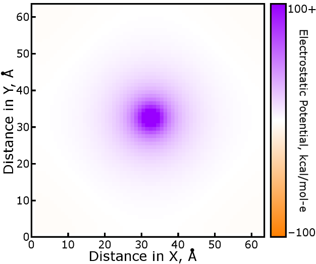
As would be expected, the shape of the potential is roughly circular (spherical in three dimensions), but not quite: if the box were much smaller it would become apparent in the image. The potential is a lot like kq_iq_j erf(αr_ij) / r_ij, but not quite: the nature of the B-splines in Fourier space can be examined by returning additional arguments from pmeOrthoConvBC. Of course, nowhere is the pair potential negative, but individual charges can be and will scale it accordingly.

The code should make clear that this pair potential is an analytic result obtained for a particular box size and mesh dimensions. The result U could be stored, pre-transformed by 3DFFT even, for inclusion in the convolution of any charge mesh with the same dimensions. In fact, this could save some time in the reciprocal space calculation but it's trivial in the grand scheme of things. The analytic approach is nice because, if the simulation box size changes, the pair potential will automatically update.

The pair potential above is the key to understanding why PME, even with the FFT, is a fundamentally pairwise operation. The FFT merely makes it a lot faster for dense systems of particles. For the 4^th order interpolation in this example, the 64-element stencils projecting each of two charges onto the charge grid would interact according to this potential (even if those stencils overlap‐note that the potential is not infinite even at (32,32,32)), implying 4096 table lookups to compute the long-ranged component of the particles' interaction in a pairwise sense.

An understanding of this material may make it more comfortable to get into the &ewald namelist of sander or pmemd job control files. There are still a number of algorithmic constraints that limit the options that can take effect in the workhorse, GPU version of pmemd (the grid size must be a multiple of 4, for example), but that may improve with time. More broadly, this demonstration aims to teach the methods behind particle-particle, particle-mesh techniques, which have applications throughout computational physics. Any questions or comments may be forwarded to david.cerutti (at) rutgers.edu.

Go to the previous section