(Note: These tutorials are meant to provide illustrative examples of how to use the AMBER software suite to carry out simulations that can be run on a simple workstation in a reasonable period of time. They do not necessarily provide the optimal choice of parameters or methods for the particular application area.)
Copyright Ross Walker 2013

Using Accelerated Molecular Dynamics (aMD) to enhance sampling SECTION 3

Formerly known as AMBER Advanced Tutorial 22

By Romelia Salomon, Levi Pierce & Ross Walker

3) Analyzing the aMD results

The final stage of our calculation is to use cpptraj and other tools to analyze the results of our aMD calculations.

The plot on the right shows a projection on the first two PCA vectors of the trajectory obtained from our 500ns aMD run. As a reference the middle plot shows a 500ns simulation on AMBER using the same files and running parameters, but using only conventional MD instead of aMD projected onto our aMD PCA space. Finally the left plot shows the projection of the trajectory from the very long run from DE Shaw's and co-workers onto our aMD PCA vectors.

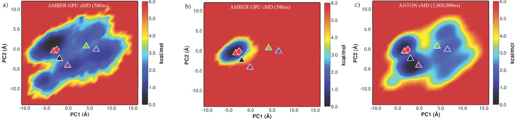
This plots show how a relatively short aMD simulation run on AMBER GPU version, allowed us to sample an equivalent phase space than a very long and very impressive run on Anton by the DE Shaw research group. The cpptraj input file used to produce the PCA vectors from the aMD trajectory and further project this trajectories onto the produced PCA vectors is included here.

AMD/bpti/protein_amd_all.nc 1 last 1

reference AMD/bpti/bpti.inpcrd

center origin :1-58

image origin center

strip :WAT,Cl-

rms reference mass :1-58@CA,C,N out AMD/bpti/pca-analysis/PDBfit/RMSD.out

matrix covar name matrixdat @CA out covmat-ca.dat

analyze matrix matrixdat out evecs-ca.dat vecs 174

analyze matrix matrixdat name evecs-ca vecs 174

analyze modes fluct out analyzemodesflu.dat stack evecs-ca beg 1 end 174

analyze modes displ out analyzemodesdis.dat stack evecs-ca beg 1 end 174

projection modes evecs-ca.dat out pca12-ca beg 1 end 3 @CA

go

The command line to run this file through cpptraj is the following:

cpptraj < ptraj.in > ptraj.out

Similarly, to project either the 500ns conventional MD trajectory from AMBER, or the 1ms trajectory from DE Shaw we used an input file like the following. First the trajectory is aligned and printed out in a binpos format.

reference ../scratch.md99SBi/av-CA.pdb
trajin shaw1-CA.pdb
trajin shaw2-CA.pdb
trajin shaw3-CA.pdb
trajin shaw4-CA.pdb
trajin shaw5-CA.pdb
trajin xray-CA.pdb
trajin BPTI-SHAW/DESRES-Trajectory-bpti-c-alpha/bpti-c-alpha/bpti-c-alpha-000.dcd 1 -1 2
...
trajin BPTI-SHAW/DESRES-Trajectory-bpti-c-alpha/bpti-c-alpha/bpti-c-alpha-041.dcd 1 -1 2
rms reference out rms-av.dat :4-54@CA
trajout alav-CA.bps binpos nobox
go

Then, the produced trajectory is projected on the previously produced PCA vectors, we used the first three in our case.

trajin alav-CA.bps
projection modes ../scratch.aMD-C67-NEW-first500ns/evecs-ca.dat out pca12-ca beg 1 end 3 :4-54@CA
go

4) Reweighting the aMD results

One of the main advantages of aMD is the possibility of reweighting the distribution obtained in a simulation to recover the unperturbed one. During an aMD simulation an amd.log file is created. The amd.log file contains all the information you need to do reweighting, it gets written with the same frequency at which the configurations are saved to disk in the trajectory file. Each line corresponds to the information of a corresponding snapshot being saved on the mdcrd file. Regardless of what iamd value is used, the number of columns in the amd.log file are always the same, they just have 0 or 1 (correspondingly) if no boost is being added to dihedral or total energy

The amd.log file has the following header:

#All energy terms stored in units of kcal/mol

#ntwx,total_nstep,Unboosted-Potential-Energy, Unboosted-Dihedral-Energy,Total-Force-Weight,Dihedral-Force-Weight,Boost-Energy-Potential,Boost-Energy-Dihedral

The description for the main columns is as follows:

a) Unboosted-Potential-Energy = Total Potential Energy without boost added, kcal/mol

b) Unboosted-Dihedral-Energy = dihedral energy without boost added, kcal,mol

c) Total-Force-Weight = The force scaling factor calculated from the boost to the Total Potential Energy

d) Dihedral-Force-Weight = The dihedral force scaling factor from dihedral boost

e) Boost-Energy-Potential = The boost energy in kcal/mol

f) Boost-Energy-Dihedral = The dihedral boost energy in kcal/mol

IMPORTANT NOTE:

Before Amber 14 the boost energy for the dihedral and total potential energy (last two columns) was given in units of KT. This decision was made at the beginning with the idea that the user could read and use these values directly for reweighting without any further work, but later it we decided it was much better and more consistent to have all energy output in kcal/mol as the rest of AMBER's energy output. As of AMBER 14, the last two columns of the amd.log file as given in units of kcal/mol.

For reweighting aMD results we would like to add the link to a great tutorial (aMD reweighting tutorial) which also provides a small python script to performs the reweighting. The script is compatible with the newer versions of AMBER (12 through 14) and can be used to reweight 1D and 2D distributions. We also include here a simple C code that performs 2D aMD reweight based on the Kernel Density Estimation algorithm reweight-KDE.c . This algorithm also performs very well and reduces the amount of noise without using a truncated expression for the exponential. The function has couple parameters that can b adjusted, but are documented in the reweight-KDE.c file.

To reweight a 2D distribution, like our PCA plot or a common Phi-Psi distribution, a file containing the 2D information for each frame has to be generated. For a Phi_Psi distribution file, AmberTools can be used. For example, for dipeptide alanine phi-psi distribution:

# 2 ALA PHI: (1 ACE C)-(2 ALA N)-(2 ALA CA)-(2 ALA C) -180 -180

# dihedral iat 5, 7, 9, 15,

dihedral phi :1@C :2@N :2@CA :2@C out Phi_Psi

# 2 ALA PSI: (2 ALA N)-(2 ALA CA)-(2 ALA C)-(3 NME N) -180 -180

# dihedral iat 7, 9, 15, 17

dihedral psi :2@N :2@CA :2@C :3@N out Phi_Psi

go

Remove the first line, header, if using the reweight-KDE.c routine. Also a file containing the aMD weights needs to be generated by extracting the proper information from the amd.log file. This can easily be done with the following command:

# For AMBER14:

# awk 'NR%1==0' amd.log | awk '{print ($8+$7)/(0.001987*300)" " $2 " " ($8+$7)}' > weights.dat

# For AMBER12:

# awk 'NR%1==0' amd.log | awk '{print ($8+$7)" " $3 " " ($8+$7)*(0.001987*300)}' > weights.dat

After both files have been created, you can use either the python script or this simple c code.

For instance for the python code:

python PyReweighting-2D.py -input Phi_Psi -Emax 100 -discX 6 -discY 6 -job amdweight_MC -order 10 -weight weights.dat | tee -a reweight_variable.log

For the reweight-KDE.c program, compile and run:

gcc reweight-hammelberg.c -o reweight-hammelberg -lm

./reweight-KDE

Both options produce good quality reweight distributions and generate output files that can be visualized with gnuplot or some other similar program.

One of the reasons we chose BPTI is that it has been experimentally studied extensively. Further analysis of the aMD trajectory can be found in our paper Levi C.T. Pierce, Romelia Salomon-Ferrer, Cesar Augusto F. de Oliveira, J. Andrew McCammon, and Ross C. Walker. "Routine Access to Millisecond Time Scale Events with Accelerated Molecular Dynamics". J Chem Theory Comput. 2012 September 11; 8(9): 2997-3002. We will not include the rest of the analysis as is it not essential to run aMD.

RETURN TO INDEX