SECTION 3: Linear interaction energy analysis
FEW
provides the functionality to conduct binding free energy calculations
according to the linear interaction energy (LIE) approach
described in detail in
[3,
4].
In this approach the binding free energy is estimated from the change
in electrostatic (ele) and
van der Waals (vdW) interaction energy between the ligand and its
environment upon complex formation.
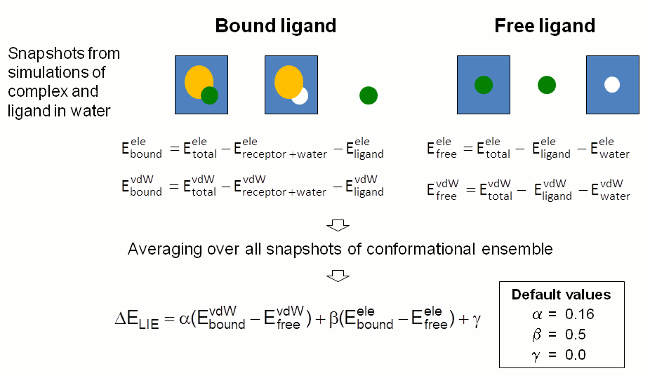
The interaction energy contributions are determined from snapshots of
MD simulations of the
free and the complex bound ligand in solution by subtracting the
energies of the individual components from the total energy of the
solvated systems (Figure 4). Energies are determined by single point
calculations with sander.
The interaction energies calculated for individual
snapshots are averaged over the whole conformational ensemble selected
for evaluation
by the user.
The binding free energy is estimated as the sum of the differences in
vdW and electrostatic
interaction energies scaled by weighting factors (cf. last equation in
Figure 4). FEW uses
established weighting factors to provide a rough estimate of the
binding free energy of a
ligand for the studied target system.
 |
| Figure 4: Schematic depiction of procedure employed in FEW for the estimation of the ligand binding free energy by the LIE approach. |
Prerequisite for the setup of LIE analyzes with FEW is the existence of trajectories of the ligand and the complex in solution generated using the MD setup functionality of FEW. As we have already created such trajectories in section 1 of the tutorial employing the 3-trajectory setup for MM-PBSA calculations, all necessary information is already available. As command-file for the preparation of the LIE analyzes serves the file lie_am1 located in the /home/user/tutorial/cfiles directory.
Tip: If you plan to conduct only LIE calculations, setup the MD simulations with traj=3 and use LIE instead of MMPBSA in the FEW program call. This way only MD simulations for complex and ligand are prepared and no receptor simulation, which is superfluous for LIE analyzes, is setup.| lie_am1 |
| @LIEW ################################################################################ # Command file for LIE calculations based on trajectories # generated by molecular dynamics simulations previously. ################################################################################ # Location and features of input and output directories / file(s) # # lig_struct_path: Folder containing the ligand input file(s) # output_path: Basis directory in which all setup and analysis folders will # be generated. The directory needs to be identical with the # 'output_path' directory used for setup of the MD simulations. lig_struct_path /home/user/tutorial/structs output_path /home/user/tutorial # Receptor features # water_in_rec: Water present in receptor PDB structure # used for setup of MD simulations water_in_rec 1 ################################################################################ # General Parameters for LIE calculation setup # # lie_calc: Request setup of LIE calculations # charge_method: Charge method used for MD, either "resp" or "am1" # no_of_rec_residues: Number of residues in receptor structure # additional_library: If an additional library file is required, e.g. for # non-standard residues present in the receptor structure, # this file must be specified here. # additional_frcmod: If additional parameters are needed, e.g. for describing # non-standard residues present in the receptor structure, # a parameter file should be provided here. # lie_executable: Location of LIE calculation script provided with FEW. # If no script is specified, it is assumed that the LIE # program is located in the default directory. # lie_batch_template: Template batch file for LIE calculation # lie_batch_path: Path to regard as basis path for setup of batch files # lie_calc 1 charge_method am1 no_of_rec_residues 290 additional_library /home/user/tutorial/input_info/CA.lib additional_frcmod lie_executable lie_batch_template /home/user/tutorial/input_info/lie.sge lie_batch_path # ################################################################################ # Parameters for coordinate extraction # # image_trajectories: If set to "1" solutes of the specified trajectories # will be imaged to the origin before coordinates are # extracted. Please regard that this may require a large # amount of additional disc space. # trajectory_files: Trajectory files to regard. The path will be determined # automatically. Specify 'all' to regard all trajectories # produced in the production phase of the MD simulations. # This ensures consistent snapshot numbering. # Subsets of snapshots will be generated according to the # parameters first_lie_snapshot, last_lie_snapshot, and # offset_lie_snapshots. If only a subset of the trajectories # from MD shall be used, the individual files must be # specified as 'trajectory_file # entry per line. # ATTENTION: The trajectory file(s) must exist for both the # simulation of the complex and the simulation of # the free ligand in solution. # snaps_per_trajectory: Number of snapshots stored in each trajectory. # # trajectory_files md_prod_001.mdcrd.gz trajectory_files md_prod_002.mdcrd.gz # snaps_per_trajectory 50 ################################################################################ # LIE Analysis # # calc_sasa: Request calculation of change in solvent accessible surface area # first_lie_snapshot: No. of snapshot from which the LIE calculation # shall be started # last_lie_snapshot: No. of last snapshot that shall be regarded in the # LIE calculation # offset_lie_snapshots: Offset between snapshots that shall be regarded # in the LIE calculation # sander_executable: Sander executable that shall be used for the LIE # calculation, if this differs from the default one # in $AMBERHOME/bin # parallel_lie_call: Call for running sander in parallel, e.g.: # mpirun -np 2 -machinefile $PBS_NODEFILE # Prerequisite: Parallel version of sander installed # delete_lie_trajectories: Delete trajectory files created for LIE analysis # directly after energy calculation # calc_sasa 0 first_lie_snapshot 81 last_lie_snapshot 100 offset_lie_snapshots 1 sander_executable parallel_lie_call mpirun -np 8 delete_lie_trajectories 0 |
The FEW command-file for LIE analyzes consists of the following parts:
1. Location of input and output directories / file(s):
Here the input / output specific parameters are defined. This part of
the script is identical with
the corresponding part
of the other command files presented before (see e.g. section 1).
2. General Parameters for LIE calculation setup:
LIE analyzes are setup based on MD simulations in which
am1
charges
were used for the ligand(s). For the
structurally bound calcium ion of the
290
residues
comprising receptor an additional library file is loaded. The
LIE.pl
executable
is assumed to be in the default location
and LIE calculations are setup using the
basic input/output directory
as output directory. As template for
the setup of batch files servers the file specified under
lie_batch_template.
In
this template file the settings before the
Prepare
calculation
section
need to be adapted to the computing environment
where the LIE calculations shall be performed.
3. Parameters for coordinate extraction:
This part of the command file is similar to the snapshot
extraction specific part of the command file for MM-PB(GB)SA
calculations described in section 2
of this tutorial. Imaging of the trajectories before coordinate
extraction is requested. All
trajectories that have been produced during MD production are
specified. This is required to ensure correct identification of the
snapshot coordinates.
The snapshots that shall be taken into account in
the LIE calculations are selected based on
the number of snapshots present in each trajectory file
snaps_per_trajectory
as
well as based on
first_lie_snapshot,
last_lie_snapshot, and
offset_lie_snapshots in section 4
described below.
4. Parameters for LIE analyzes:
LIE analyzes are requested based on snapshots
81
to
100
with
an
offset
of
1.
FEW
offers the possibility to compute the difference in the solvent
accessible surface area of the ligand between the bound and the free
state, since this
quantity has been used to determine a ligand specific coefficient
γ (cf. last equation in Figure 4)
[8,
9,
10].
Here,
however, this option is not selected
(calc_sasa=0).
A
computing environment specific
parallel_lie_call
for sander
is provided. Consequently the LIE analyzes will be
run with the parallel version of sander
under
$AMBERHOME/bin/sander.MPI.
As
the trajectories that are generated for LIE analysis
from the original MD trajectories contain water
molecules explicitly and can therefore consume a large amount of disk
space, FEW offers to delete them directly
after the LIE calculation for one ligand has been completed. This
option was not switched on here
(delete_lie_trajectories=0).
Running
FEW:
When the computing environment specific settings have been adapted and
the
basic input/output path
in
the command file has been correctly specified, the LIE calculations
can be prepared with FEW.
The
output:
After successful termination of FEW, the
/home/user/tutorial
directory
contains a new folder called
lie_am1
with
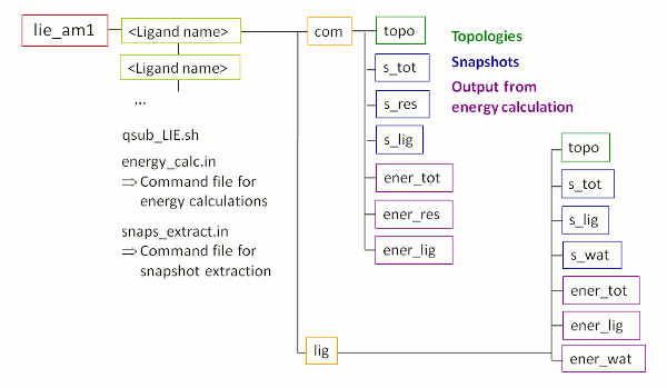
the sub-structure shown in Figure
5. Please note, the energy calculation folders depicted in
violet in
Figure 5 are not present yet. They will be created during the LIE
calculations.
 |
| Figure 5: Schematic depiction of sub-structure of the folder created upon LIE analysis using FEW. |
Starting the LIE calculations:
LIE calculations can be started by executing the shell script qsub_LIE.sh located in the lie_am1 folder.
/home/user/tutorial/lie_am1/qsub_LIE.sh
LIE results:
The final results of the LIE calculations can be found in the ligand specific sub-folders of the /home/user/tutorial/lie_am1 directory. The file LIE_s<S>_<T>_<O>.txt with <S> = first_lie_snapshot, <T> = last_lie_snapshot, and <O> = offset_lie_snapshots, i.e. in case of this tutorial the file LIE_s81_100_1.txt, lists the calculated average electrostatic and vdW interaction energies (and the solvent accessible surface area) for the complex bound and the free ligand, as well as their differences. Furthermore an estimate of the binding free energy using the scaling factors shown in Figure 4 is given.
| Result file LIE_s81_100_1.txt of ligand L51c |
|
Energy contributions: Mean energy Standard deviation Standard error Complex non-bonded VDW: -76.550390 3.354497 0.750088 Complex non-bonded ELE: -49.058070 7.613551 1.702442 Ligand non-bonded VDW: -43.399665 3.762162 0.841245 Ligand non-bonded ELE: -56.828235 6.755975 1.510682 ================================================================================ Final LIE results: Differences in interaction energies and SASA: Delta electrostatic energy (dE-ele): 7.770165 kcal/mol Delta van der Waals energy (dE-vdW): -33.150725 kcal/mol ________________________________________________________________________________ Estimated binding free energy: ATTENTION: Please note that the estimate of the binding free energy (dG-bind) provided below was calculated according to the equation dG-bind = alpha * dE-vdW + beta * dE-ele with fixed coefficients of alpha=0.16 and beta=0.5. We strongly recommend to thoroughly investigate whether using other coefficients could be beneficial in the specific case. Binding energy estimate (dG-bind): -1.419034 kcal/mol |
Tip: If you wish to determine by a linear fit the best weighting coefficients for a data set for which experimental binding affinities are known, you can extract the differences in electrostatic and vdW interaction energies (as well as the solvent accessible surface area) from all result files of a dataset with the script extract_LIEenergies.pl provided with FEW. Please refer to the FEW manual for details.
SECTION 2: MM-PB(GB)SA calculations
Copyright: Nadine Homeyer 2014


