


SECTION 2: MM-PB(GB)SA calculations
FEW
allows to prepare implicit solvent molecular mechanics calculations
according to the MM-PBSA and the MM-GBSA approach. Prerequisite for the
setup of MM-PB(GB)SA calculations is the existence of MD trajectories
in the MD simulation folders generated with help of the MD setup
functionality of FEW (see steps 1A
& 1B
of this tutorial). FEW allows to prepare MM-PB(GB)SA calculations
according to both
the 1-trajectory and the 3-trajectory approach [1].
Here we will apply both alternatives to the three Factor Xa inhibitors
for which MD simulations have been prepared in section 1 of the
tutorial
(Table
1).
For a basic introduction to the MM-PB(GB)SA method please consult the literature and Tutorial A3. The basic principles of the calculation of the binding free energy ΔGbind,solv explained in Tutorial A3 apply also for the calculations conducted here. However, since it is assumed that the change in configurational entropy of the ligands upon binding does not differ significantly, the entropic contribution to binding is not taken into account. Therefore we refer here to the binding energy computed by MM-PB(GB)SA calculations setup with FEW as effective binding energy, ΔGeffective.
Please note: The sample MM-PB(GB)SA calculations conducted here are based on snapshots from the 2 ns MD simulations prepared in section 1 of the tutorial. Therefore it cannot be expected that the snapshots used for the calculations represent fully equilibrated structures. In addition the small number of considered snapshots further increases the uncertainty of the predictions. Consequently the MM-PB(GB)SA calculations shown here should only be regarded as an example for demonstrating the functionality of FEW. For any "real-life" study it is highly recommended to thoroughly analyze the MD trajectories to identify representative structural ensembles for the MM-PB(GB)SA calculations, because only MM-PB(GB)SA calculations conducted based on such ensembles can result in accurate binding energy predictions. Some basic analyzes for the investigation of the equilibration status can be found in Tutorial A3, section 2.
A: 3-trajectory approach
Since we have setup and run MD simulations according to the 3-trajectory approach in section 1, we can directly start with the setup of the MM-GBSA, 3-trajectory approach calculations using the FEW command file ana_am1_3trj_pb0_gb2.| mmpbsa_am1_3trj_pb0_gb2 |
| @WAMM ################################################################################ # Command file for MM-PBSA / MM-GBSA calculations based on trajectories # generated by molecular dynamics simulations previously. ################################################################################ # Location and features of input and output directories / file(s) # # lig_struct_path: Folder containing the ligand input file(s) # output_path: Basis directory in which all setup and analysis folders will # be generated. The directory needs to be identical with the # 'output_path' directory used for setup of the MD simulations. lig_struct_path /home/user/tutorial/structs output_path /home/user/tutorial # Receptor features # water_in_rec: Water present in receptor PDB structure # used for setup of MD simulations water_in_rec 1 ################################################################################ # General Parameters for MM-PBSA / MM-GBSA calculation setup # # mmpbsa_calc: Setup MM-PBSA / MM-GBSA calculations # 1_or_3_traj: "1" or "3" trajectory approach # charge_method: Charge method used for MD, either "resp" or "am1" # additional_library: If an additional library file is required, e.g. for # non-standard residues present in the receptor structure, # this file must be specified here. # additional_frcmod: If additional parameters are needed, e.g. for describing # non-standard residues present in the receptor structure, # a parameter file should be provided here. # mmpbsa_pl: Path to mm_pbsa.pl script mmpbsa_calc 1 1_or_3_traj 3 charge_method am1 additional_library /home/user/tutorial/input_info/CA.lib add_frcmod mmpbsa_pl $AMBERHOME/bin/mm_pbsa.pl ################################################################################ # Parameters for coordinate (snapshot) extraction # # extract_snapshots: Request coordinate (snapshot) extraction # snap_extract_template: Template file for extraction of coordinates from # trajectory, i.e. input-file for mm_pbsa.pl; only # required if non-standard input-file shall be used. # image_trajectories: If set to "1" solutes of the specified trajectories # will be imaged to the origin before coordinates are # extracted. Please regard that this may require a large # amount of additional disc space. # trajectory_files: Trajectory files to regard. The path will be determined # automatically. Specify 'all' to regard all trajectories # files produced in MD. This ensures consistent snapshot # numbering. Subsets of snapshots will be generated according # to the parameters first_snapshot, last_snapshot, and # offset_snapshots. If only a subset of the available MD # trajectories shall be used, the individual files must be # specified as 'trajectory_files # one entry per line. # first_snapshot: First structure that shall be extracted from trajectory # last_snapshot: Last structure that shall be extracted from trajectory # offset_snapshots: Frequency of structure extraction # image_trajectories 1 # trajectory_files all # first_snapshot 1 last_snapshot 100 offset_snapshots 1 ################################################################################ # MM-PBSA / MM-GBSA Analysis # mmpbsa_template: Template file for MM-PBSA / MM-GBSA analysis - File used # as input-file for mm_pbsa.pl; only required if non-standard # file shall be used. # PB: If not zero PB calculation will be performed # Options: "0" -> No PB # "1" -> PB with calculation of the non-polar part of the # solvation free energy using the Method developed by # Tan et al. (J. Phys. Chem. B, 2007, 111, 12263-12274). # This method can only be run in combination with GB=1 # or GB=0. # "2" -> Hybrid model developed by H. Gohlke and A. Metz # with IVCAP=5 and CUTCAP=50 # "3" -> PB with MS=1 and Parse radii # "4" -> PB with MS=1 and mbondi radii. This method can only # be combined with GB=1 or GB=0. # GB: If not zero GB calculation will be performed # Options: "0" -> No GB # "1", "2", "5" -> GB analysis according to 'igb' (see manual) # # decomposition: If larger 0 energy decomposition of specified type is # performed. Options: 1-4 - See Amber manual for decomposition # type options. Decomposition only works with PB=4 and GB=1. # SASA is calculated by the ICOSA method. # no_of_rec_residues: Number of residues in the receptor structure # # total_no_of_intervals: Total number of intervals to analyze. # The total_no_of_intervals needs to be consistent with # the number of 'first_PB_snapshot', 'last_PB_snapshot', # and 'offset_PB_snapshots' definitions below. Setting # total_no_of_intervals to a value larger than 1, is # usually only necessary if snapshots with different # offsets shall be analyzed. # first_PB_snapshot: Structure to start analysis with # last_PB_snapshot: Last structure to regard in analysis # offset_PB_snapshots: Specification of offset between structures that shall # be regarded in the MM-PBSA calculation # # mmpbsa_batch_template: Batch script template for MM-PBSA calculation # mmpbsa_batch_path: Optional, path to regard as basis path for batch script # setup, in case it differs from mmpbsa_template PB 0 GB 2 # decomposition 0 no_of_rec_residues 290 # total_no_of_intervals 1 first_PB_snapshot 51 last_PB_snapshot 100 offset_PB_snapshots 1 # mmpbsa_batch_template /home/user/tutorial/input_info/MMPBSA.sge mmpbsa_batch_path /home/user/tutorial # mmpbsa_sander_exe parallel_mmpbsa_calc 1 |
The command file consists of the following parts:
1.
Location of input and output directories / file(s):
Identical with the input/output information part discussed in section 1
of this tutorial.
2.
General Parameters for MM-PBSA / MM-GBSA calculation setup:
MM-GBSA calculations are prepared according to the 3-trajectory approach
(1_or_3_traj=3).
using
MD trajectories generated with ligand atomic charges determined
by the AM1-BCC method. For the setup of the topology files without
water the additional library file for
calcium ions is employed again and the MM-GBSA analyzes are conducted
with the mm_pbsa.pl script located in the bin
directory
of the local AMBER installation.
3.
Parameters for coordinate (snapshot) extraction:
It is requested that after imaging snapshots 1 to 100 are extracted
without offset between the snapshots
(offset_snapshots=1) from
the 2 ns trajectories generated in section 1 of this tutorial.
4.
MM-PBSA / MM-GBSA Analysis:
MM-GBSA calculations according the method of Onufriev et al. 2004
[6]
corresponding to igb=2
in
AMBER12 are requested. Structurally bound ions are considered as
part of the receptor here, so that the total number of receptor
residues amounts up to 290. Calculations
are run for snapshots 51
to 100 with an offset of 1.
Computing parameters are set such that
mm_pbsa.pl
will
be run in serial using the
/home/user/tutorial
directory
as
basic input/output directory
directory.
The batch script
MMPBSA.sge
is
used as template batch file for job submission.
Please modify the header section of this script before the
Prepare
calculation
section
according to your computing environment architecture.
Running FEW:
When you have ensured that the path of the basic input/output directory is specified correctly in the command file, setup of the MM-GBSA calculations by FEW can be invoked by:
$FEW/FEW.pl MMGBSA /home/user/tutorial/cfiles/mmpbsa_am1_3trj_pb0_gb2
The output:
After successful completion of the FEW run, a new folder called calc_a_3t exists in the basic input/output directory, i.e. the tutorial, directory. This calc_a_3t folder (Figure 3), which is named after the procedure employed (a = am1 and 3t = 3-trajectory approach), contains a sub-folder for each ligand in which the topologies without water (topo), the extracted snapshots (snapshots), and the input-files for the MM-GBSA calculation (s51_100_1) are located.
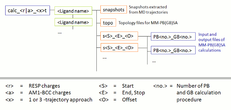 |
| Figure 3: Schematic depiction of sub-structure of the folder for MM-PB(GB)SA calculations created by FEW. |
To start the MM-GBSA calculations execute the qsub_s51_100_1_pb0_gb2.sh script located in the calc_a_3t folder.
/home/user/tutorial/calc_a_3t/qsub_s51_100_1_pb0_gb2.shThe result files of the calculations appear in the folder
/home/user/tutorial/calc_a_3t/<ligand name>/s51_100_1/pb0_gb2
As looking up the individual results for all ligands can be work extensive, if ten or more ligands are studied, a script is distributed with FEW that allows an automated extraction of the final ΔGbind,effective values and the individual ΔE contributions. The script requires a text file in which the names of the ligands that shall be regarded are specified (one name per line), e.g.:
File: structs.txt
L51c
L51d
L51g
perl $FEW/miscellaneous/extract_WAMMenergies.pl structs.txt /home/user/tutorial/calc_a_3t pb0_gb2 51_100_1
The last term corresponds to first_PB_snapshot, last_PB_snapshot and offset_PB_snapshots separated by "_". After termination of the run, you will find a script called pb0_gb2.txt in the /home/user/tutorial/calc_a_3t folder, that summarizes the final results (see below).| pb0_gb2.txt |
| Ligand ELE VDW NP_SOLV P_SOLV E_TOT L51c -192.36 -64.05 -4.80 189.55 -59.35 L51d -30.70 -62.01 -2.52 36.15 -48.68 L51g -103.96 -76.04 -4.92 113.28 -66.07 |
The energetic contributions given in this file correspond to the changes in energy upon ligand binding, i.e. complex formation, for:
- ELE Electrostatic energy
- VDW Van der Waals interaction
- NP_SOLV Non-polar contribution to solvation free energy
- P_SOLV Polar contribution to solvation free energy
- E_TOT Total binding energy, i.e. ΔGeffective
/home/user/tutorial/calc_a_3t/L51c/s51_100_1/pb0_gb2/L51c_statistics.out.snap
you see that the ΔGeffective values calculated for the individual snapshots reach from ca. -165.6 to +84.07 kcal/mol. Consequently the standard deviation is quiet high (60.8 kcal/mol). One factor that significantly contributes to the large fluctuations in the calculated energies is the noise in the internal energies. In the 3-trajectory approach the internal energies of complex, receptor, and ligand do not cancel, so that even small differences between the structures can have large effects on the calculated binding energies. This noise is avoided in the 1-trajectory approach, in which binding energies are calculated exclusively based on structures of the complex, disregarding the free forms of ligand and receptor.B: 1-trajectory approach
Despite the fact that in the so-called 1-trajectory approach only structures from a simulation of the complex are taken into account and the structural differences of the unbound versus the bound receptor and ligand are thus not considered, this approach is often applied and has shown to be capable to yield good relative binding energy predictions. A great advantage of this approach is that it is less computationally demanding, because only a MD simulation of the complex needs to be conducted. In addition it benefits from the cancellation of internal energy contributions which leads to less noisy ΔE values.Thus, as the 1-trajectory approach is often used for the estimation of relative ligand binding energies, the setup of MM-PB(GB)SA calculations according to this approach is also demonstrated here. The general proceeding is equivalent to the one shown for the 3-trajectory approach above. We can proceed as in step 2A. First create a command file for FEW called mmpbsa_am1_1trj_pb3_gb0 which is identical to the mmpbsa_am1_3trj_pb0_gb2 file shown above. Then set 1_or_3_traj=1, GB=0, and PB=3. As now computationally more expensive Poisson-Boltzmann calculations will be performed, the number of considered snapshots can be reduced by setting first_PB_snapshot=81 to save computing time. If you now run FEW with this command file, you will obtain input files for MM-PBSA calculations with Parse radii according to the 1-trajectory approach. The final results of these calculations are shown below. Despite the short simulation time, the small number of snapshots considered, and the approximations made by the 1-trajectory approach, the computed binding energies ΔGeffective (E_TOT) show for all ligands the expected trend (cf. Table 1).
| pb3_gb0.txt |
| Ligand ELE VDW NP_SOLV P_SOLV E_TOT L51c -19.05 -61.20 -6.20 61.16 -25.28 L51d -20.54 -64.81 -6.27 69.46 -22.17 L51g -21.64 -65.20 -6.28 66.50 -26.62 |
Copyright: Nadine Homeyer 2014