


Electrostatic Parameterization with py_resp.py
This tutorial is compatible with AmberTools23 or later versions. If you are using an earlier version of AmberTools, please update to the latest version.
Learning Outcomes
- Understand the limitations of additive force fields and the need for polarizable models like pGM-ind and pGM-perm.
- Learn about the steps involved in the parameterization process of the PyRESP algorithm
- Learn how to perform QM geometry optimization using Gaussian.
- Learn how to calculate the electrostatic potential (ESP) surrounding the molecule using Gaussian.
- Understand the format conversion of Gaussian ESP data for pyresp_gen.py and py_resp.py to read.
- Learn how to perform RESP, pGM-ind, and pGM-perm parameterizations using pyresp_gen.py and py_resp.py.
- Understand the differences between the three electrostatic models in terms of atomic charges and induced/permanent dipole moments.
- Analyze the output files to assess the quality of fitting for each model.
Introduction
In this tutorial, we will work through the usage of pyresp_gen.py and py_resp.py for electrostatic parameterizations for pyridoxal phosphate (PLP). PLP is the active form of vitamin B6, which is a coenzyme in a variety of enzymatic reactions. At the time of this writing, PLP presents in more than 200 Protein Data Bank (PDB) entries as a standalone ligand, and more than 1,000 PDB entries as a covalently linked ligand. py_resp.py is a Python program extending the functionalities of the ancestor program resp, and pyresp_gen.py is a Python program that automates the generation of input files for py_resp.py. See the Amber Reference Manual for introductions of the two programs.
The RESP (Restrained ElectroStatic Potential) algorithm fits the quantum mechanically (QM) calculated molecular electrostatic potential (ESP) at molecular surfaces using an atom-centered point charge model, which is compatible with additive Amber force fields such as ff19SB, ff14SB, and gaff2. Refer to J. Phys. Chem. 1993, 97, 40, 10269–10280 for details of the RESP algorithm and here for a tutorial for the usage of the resp program. However, the additive force fields are unable to model the important atomic polarization effects. Several induced dipole based polarizable models have been incorporated into Amber, such as the polarizable Gaussian Multipole (pGM) force field described in page 407 of Amber 2023 manual that is still under active development. py_resp.py provides electrostatic parameterization schemes for the RESP model with atomic charges for the additive force fields, and the pGM-ind and pGM-perm models with additional induced and permanent dipole moments. For details of the py_resp.py program and the PyRESP algorithm, please see J. Chem. Theory Comput. 2022, 18, 6, 3654–3670.
As the RESP procedure, the parameterization using the PyRESP procedure consists of 3 steps. First, we need to optimize the geometry of the molecule to be parameterized, then we need to generate electrostatic potential surrounding the molecule, and then finally we need to run the PyRESP parameterization. In this tutorial, we will show the electrostatic parameterization of PLP with three models: RESP, pGM-ind, and pGM-perm. All QM calculations will be performed using Gaussian.
Process
-
QM Geometry Optimization
First, we obtain the idealized structure of PLP in SDF format from https://files.rcsb.org/ligands/download/PLP_ideal.sdf. You can also download the idealized structure of PLP here.
Fig. 1 is the idealized structure of PLP viewed using visualizer software Avogadro. Note that in physiological condition, the phosphate group should be deprotonated. Therefore, we remove the two hydrogen atoms attached to the phosphates group (selected atoms displayed in cyan spheres in Fig. 1).
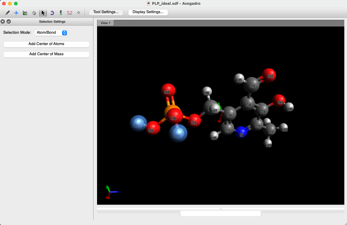
Fig.1. Idealized structure of PLP.
Next, we generate the Gaussian input files for QM geometry optimizations. Consistent with the original PyRESP paper, we use B3LYP/6-311++G(d,p) level of theory. For convenience, we use a single conformation of PLP for parameterization, although multiple-conformation parameterization is also supported by py_resp.py. The creation of Gaussian input files is beyond the scope of this tutorial, but they are provided below for reference. Here are the Gaussian input and output files: PLP_ideal_opt.gin, PLP_ideal_opt.gout.
We can generate the optimized coordinates in pdb format for comparison. Here we use Newzmat which ships with Gaussian to convert the checkpoint file to a pdb file.
newzmat -ichk -opdb PLP_ideal_opt.chk PLP_ideal_opt.pdb
The pdb file for optimized coordinates is provided here: PLP_ideal_opt.pdb.
-
Electrostatic Potential Calculation
The next step is to calculate the ESP surrounding the optimized PLP molecule that can ultimately be read by the py_resp.py program. Consistent with the original PyRESP paper, we use MP2/aug-cc-pVTZ level of theory. The Gaussian route line for this project needs to read:
#MP2/aug-cc-pVTZ Geom=Check SCF=Tight Pop=MK IOp(6/33=2,6/42=6,6/43=20) Guess=Read Density=Current
- Geom=Check - Read molecule coordinates from the checkpoint file of the optimized structure.
- IOp 6/33=2 - Makes Gaussian write out the potential points and the potentials. Do not change.
- IOp 6/42=6 - Specifies the point density in each layer, which is 6 points/square angstrom in this case. The number can be reduced for larger molecules or increased for small molecules.
- IOp 6/43=20 - Specifies increment between layers, which is 0.01*20=0.2 times the van der Waals radii.
Here are the Gaussian input and output files: PLP_ideal_opt_esp.gin, PLP_ideal_opt_esp.gout.
-
Convert the Gaussian ESP data format for PyRESP
py_resp.py only reads in ESP data in a specific file format. To convert from the Gaussian output format to the RESP input format, we use the espgen program ships with AmberTools:
espgen -i PLP_ideal_opt_esp.gout -o PLP_ideal_opt_esp.dat -p 1
The -p option will generate extra information such as atom types, which is necessary for the parameterization of the pGM-ind and pGM-perm models. Here is the generated dat file: PLP_ideal_opt_esp.dat.
Note if you aim to perform multiple conformation parameterizations, you can use the cat command to concatenate all generated dat files into a single file, as did in tutorial https://ambermd.org/tutorials/advanced/tutorial1/section1.php.
After obtaining the esp dat files, we will parameterize PLP for the following 3 electrostatic models: RESP, pGM-ind, and pGM-perm, which will be introduced individually. The preparation of the input files for py_resp.py can be tedious and error-prone. In particular, a “two-stage” parameterization strategy is recommended, as introduced in both the original RESP paper and PyRESP paper. For this reason, we have developed the pyresp_gen.py program for automatically generating input files for the py_resp.py program. (Manuscript in preparation) pyresp_gen.py has been included in AmberTools23. As the user, it is still recommended to read the papers understand the two-stage parameterization strategy to make sure everything is correct during the parameterization processes. More details about pyresp_gen.py and py_resp.py can be found in page 358 of Amber 2023 manual.
-
RESP Parameterization
For RESP parameterization, create a new folder named resp, and copy the generated PLP_ideal_opt_esp.dat file from step 3 into the folder. Then, we run the following script py_resp.run for executing pyresp_gen.py and py_resp.py:
#!/bin/csh -f
pyresp_gen.py -i PLP_ideal_opt_esp.dat -f1 1st.in -f2 2nd.in -p chg -q -2

echo RESP stage 1:
py_resp.py -O \
        -i 1st.in \
        -o 1st.out \
        -e PLP_ideal_opt_esp.dat \
        -s 1st.esp \
        -t 1st.chg          || goto error

echo RESP stage 2:
py_resp.py -O \
        -i 2nd.in \
        -o 2nd.out \
        -e PLP_ideal_opt_esp.dat \
        -s 2nd.esp \
        -t 2nd.chg \
        -q 1st.chg          || goto error

echo No errors detected
exit(0)

error:
echo Error: check .out and try again
exit(1)
Here are the options used for running pyresp_gen.py:
- -f1 1st.in - Specifies the name of the input for the first PyRESP stage.
- -f2 2nd.in - Specifies the name of the input for the second PyRESP stage.
- -p chg - Specifies the electrostatic model is additive point-charge model, i.e., the RESP model.
- -q -2 - Specifies the total molecular charge to be -2.
Here are the options used for running py_resp.py (stage 2):
- -i 2nd.in - Specifies the input file of general information.
- -o 2nd.out - Specifies the output file of general information.
- -e PLP_ideal_opt_esp.dat - Specifies the input file of ESP and coordinates.
- -s 2nd.esp - Specifies the output ESP file of calculated ESP values.
- -t 2nd.chg - Specifies the output parameter file.
- -q 1st.chg - Specifies replacement parameters generated from stage 1.
Here we provide the script: py_resp.run
Here are all the generated files by running the script: 1st.in, 1st.out, 1st.chg, 1st.esp, 2nd.in, 2nd.out, 2nd.chg, 2nd.esp
-
pGM-ind Parameterization
For pGM-ind parameterization, create a new folder named pgm-ind, and copy the generated PLP_ideal_opt_esp.dat file from step 3 into the folder. Then, we run the following script py_resp.run for executing pyresp_gen.py and py_resp.py:
#!/bin/csh -f
pyresp_gen.py -i PLP_ideal_opt_esp.dat -f1 1st.in -f2 2nd.in -p ind -q -2

echo RESP stage 1:
py_resp.py -O \
        -i 1st.in \
        -o 1st.out \
        -e PLP_ideal_opt_esp.dat \
        -ip $AMBERHOME/AmberTools/examples/PyRESP/polarizability/pGM-pol-2016-09-01 \
        -s 1st.esp \
        -t 1st.chg          || goto error

echo RESP stage 2:
py_resp.py -O \
        -i 2nd.in \
        -o 2nd.out \
        -e PLP_ideal_opt_esp.dat \
        -ip $AMBERHOME/AmberTools/examples/PyRESP/polarizability/pGM-pol-2016-09-01 \
        -s 2nd.esp \
        -t 2nd.chg \
        -q 1st.chg          || goto error

echo No errors detected
exit(0)

error:
echo Error: check .out and try again
exit(1)
Here is the option used for running pyresp_gen.py that is different from that of the RESP model:
- -p ind - Specifies the electrostatic model is induced dipole model, i.e., the pGM-ind model in this case.
Here is the option used for running py_resp.py that is different from that of the RESP model:
- -ip $AMBERHOME/AmberTools/examples/PyRESP/polarizability/pGM-pol-2016-09-01 - Specifies atomic polarizabilities required for the polarizable induced dipole model, which are not required for the additive RESP model.
Here we provide the script: py_resp.run
Here are all the generated files by running the script: 1st.in, 1st.out, 1st.chg, 1st.esp, 2nd.in, 2nd.out, 2nd.chg, 2nd.esp
-
pGM-perm Parameterization
For pGM-perm parameterization, create a new folder named pgm-perm, and copy the generated PLP_ideal_opt_esp.dat file from step 3 into the folder. Then, we run the following script py_resp.run for executing pyresp_gen.py and py_resp.py:
#!/bin/csh -f
pyresp_gen.py -i PLP_ideal_opt_esp.dat -f1 1st.in -f2 2nd.in -p perm -q -2

echo RESP stage 1:
py_resp.py -O \
        -i 1st.in \
        -o 1st.out \
        -e PLP_ideal_opt_esp.dat \
        -ip $AMBERHOME/AmberTools/examples/PyRESP/polarizability/pGM-pol-2016-09-01 \
        -s 1st.esp \
        -t 1st.chg          || goto error

echo RESP stage 2:
py_resp.py -O \
        -i 2nd.in \
        -o 2nd.out \
        -e PLP_ideal_opt_esp.dat \
        -ip $AMBERHOME/AmberTools/examples/PyRESP/polarizability/pGM-pol-2016-09-01 \
        -s 2nd.esp \
        -t 2nd.chg \
        -q 1st.chg          || goto error

echo No errors detected
exit(0)

error:
echo Error: check .out and try again
exit(1)
Here is the option used for running pyresp_gen.py that is different from that of the RESP and pGM-ind models:
- -p perm - Specifies the electrostatic model is induced dipole model with permanent dipoles, i.e., the pGM-perm model in this case.
Here we provide the script: py_resp.run
Here are all the generated files by running the script: 1st.in, 1st.out, 1st.chg, 1st.esp, 2nd.in, 2nd.out, 2nd.chg, 2nd.esp
-
Analysis
Among the generated files for each model, pay close attention to those generated from the 2nd stage, i.e., output parameter files named 2nd.chg, output files named 2nd.out, and output ESP files named 2nd.esp.
First, let’s focus on output parameter file 2nd.chg of each model:
For the RESP model, the atomic coordinates (%FLAG ATOM CRD) and atomic charges (%FLAG ATOM CHRG) are printed. For the pGM-ind model, beside the atomic coordinates and atomic charges sections, the atomic induced dipole moments in the global frame (%FLAG IND DIP GLOBAL) are also printed. For the pGM-perm model, beside the sections above, the atomic permanent dipole moments in both the local frame (%FLAG PERM DIP LOCAL) and the global frame (%FLAG PERM DIP GLOBAL) are printed.
Fig. 2. shows the atomic charges produced by all three models. For the RESP model, the highest positive charge is assigned to the phosphorus atom (1.4032), and the highest negative charge is assigned to the three equivalent phosphate group oxygen atoms (-0.9469). For the pGM-ind model, the highest positive charge is assigned to the formyl group carbon atom (1.0296), and the highest negative charge is assigned to the pyridine ring nitrogen atom (-2.2510). Compared with the RESP model, the magnitude of charges of most atoms are increased, due to the polarization effect considered by this model. Interestingly, the magnitude of charges of all atoms in the phosphate group are decreased. For the pGM-perm model, the highest positive charge is assigned to the formyl group carbon atom (0.9122), and the highest negative charge is assigned to the methyl group atom (-1.0593). Compared with the RESP and pGM-ind models, the charges of the pGM-perm model show very different pattern. This is because of the atomic permanent dipoles considered by this model. Fig. 3. shows the schematic representation of atomic permanent dipoles produced by the pGM-perm model, where only permanent dipoles with magnitude greater than 0.2 a.u. are displayed. Dipoles with positive values are shown in red, and dipoles with negative values are shown in blue. Note that for the phosphate group, all four oxygen atoms are assigned large dipoles pointing to the phosphorus atom, leading to the negative charge assigned to phosphorus as shown in Fig. 2.
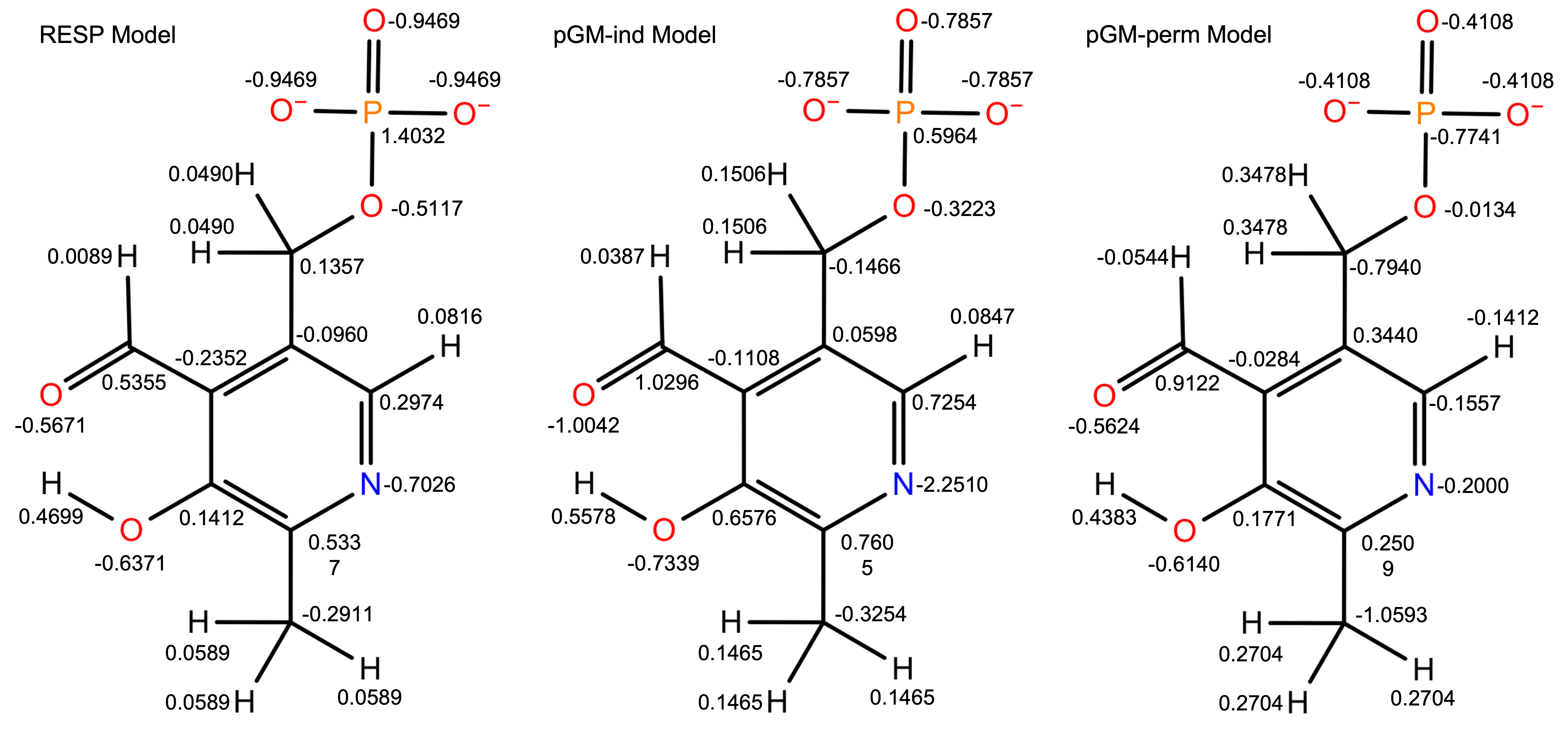
Fig.2. Atomic charges produced by all three models.
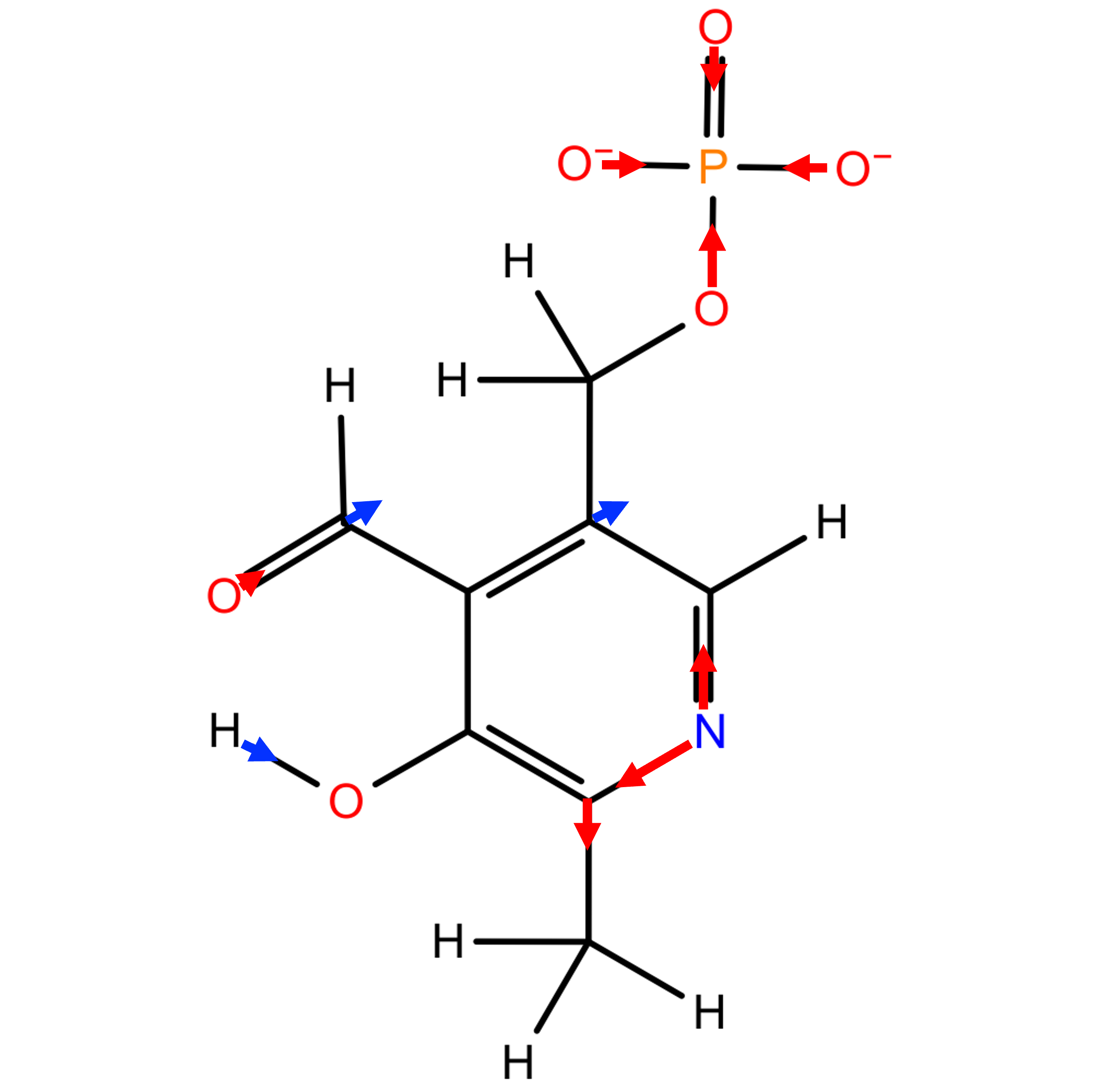
Fig.3. Schematic representation of atomic permanent dipoles greater than 0.2 a.u produced by the pGM-perm model.
Next, let’s focus on the output file 2nd.out of each model:
For this file, the Fitting Statistics Summary section and Molecular Multipole Summary section printed at the end provide useful information for assessing the quality of fitting for each model. They are summarized in Table 1.
Table.1. RRMS and Molecular Dipole/Quadrupole Moments of PLP Fitted with Each Model RESP pGM-ind pGM-perm QM RRMS 0.0110 0.0139 0.0091 Dipole Moments/Debye μ 25.5028 25.2253 25.3591 25.7419 Quadrupole Moments/Debye Angstroms Qxx 49.7113 49.5520 49.7264 49.0752 Qyy 37.1809 38.5505 37.3508 37.2835 Qzz -86.8922 -88.1025 -87.0772 -86.3587 We can see that the pGM-perm model gives the lowest RRMS value, indicating that this model gives the best fitting to QM ESPs. On the other hand, all three models give similar qualities in terms of predicting molecular dipole and quadrupole moments. Note that the QM molecular multipole moments are obtained from the PLP_ideal_opt_esp.gout file produced in step 2.
Finally, let’s focus on the output ESP file 2nd.esp of each model:
In each 2nd.esp file, the ESP values of all points calculated by QM method and each electrostatic model as well as their differences are printed in the last three columns. Using the following python script esp-fig.py, (you may need to modify file paths) we can generate the following Fig.4. showing the scatterplots of QM ESPs and ESPs calculated by each model. It can be seen that the pGM-perm model gives the best fitting to QM ESPs.
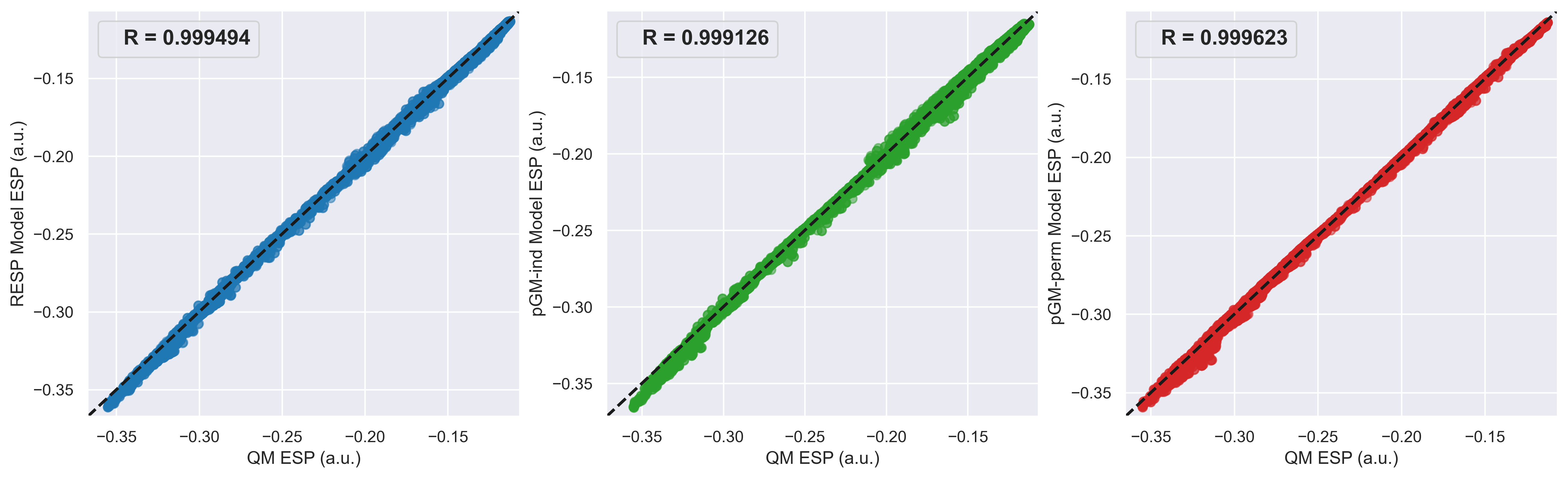
Fig.4. Scatterplots of QM ESPs and ESPs calculated by each model.
Copyright Shiji Zhao, 2023