(Note: These tutorials are meant to provide illustrative examples of how to use the AMBER software suite to carry out simulations that can be run on a simple workstation in a reasonable period of time. They do not necessarily provide the optimal choice of parameters or methods for the particular application area.)
Copyright Vinícius Cruzeiro. 2018

---

Section 3: Running and analyzing production simulations at pH 7.0 and Redox Potential -203 mV

Running the simulations

The experimental standard Redox Potential of NAcMP8 with an imidazole molecule as the axial ligand has been measured as -203 mV vs NHE and at pH 7.0 [2]. This closely represents our system (NAcMP8 with a histidine peptide axially connected), shown in the figure at the Introduction. The reference energies for the HEH residue have been fitted to reproduce this result. Therefore, when simulating our system at pH 7.0 and redox potential -203 mV we must obtain a fraction of reduced species for the HEH residue close to 50%, if the simulation is converged.

We now present the input files of the production simulations at pH 7.0 and redox potential -203 mV in both implicit and explicit solvent. In this stage, the backbone restraints are not applied. For simplicity, in this tutorial we will perform shorter production simulations than the ones performed in our publication [1]. Here, simulations are 20 ns in implicit solvent and 40 ns in explicit solvent.

For implicit solvent simulation, the command pmemd.cuda -O -i prod.implicit.mdin -p mp8_is.prmtop -c mp8_is.equi.rst7 -x mp8_is.prod.nc -inf mp8_is.prod.mdinfo -o mp8_is.prod.mdout -r mp8_is.prod.rst7 -cpin mp8_is.cpin -cpout mp8_is.prod.cpout -cprestrt mp8_is.prod.cprestrt -cein mp8_is.cein -ceout mp8_is.prod.ceout -cerestrt mp8_is.prod.cerestrt will generate the files: mp8_is.prod.mdout, mp8_is.prod.cpout, mp8_is.prod.ceout, mp8_is.prod.nc and mp8_is.prod.rst7.

For explicit solvent simulation, the command pmemd.cuda -O -i prod.explicit.mdin -p mp8_es.new.prmtop -c mp8_es.equi2.rst7 -x mp8_es.prod.nc -inf mp8_es.prod.mdinfo -o mp8_es.prod.mdout -r mp8_es.prod.rst7 -cpin mp8_es.cpin -cpout mp8_es.prod.cpout -cprestrt mp8_es.prod.cprestrt -cein mp8_es.cein -ceout mp8_es.prod.ceout -cerestrt mp8_es.prod.cerestrt will generate the files: mp8_es.prod.mdout, mp8_es.prod.cpout, mp8_es.prod.ceout, mp8_es.prod.nc and mp8_es.prod.rst7.

As can be seen above, the meaning of each input variable is explained within our input files. As the input files indicate, we may perform protonation and redox attempts at different intervals, and also perform a different number of relaxation steps in explicit solvent for successful protonation or redox state changes. In our simulations, we perform protonation and redox state change attempts in the same MD steps because ntcnstph = ntcnste. In our code, when protonation and redox state change attempts happen in the same MD step, the protonation state change attempts are performed first. In our explicit solvent simulation, the number of relaxation steps is also the same for constant pH and for contant redox potential because ntrelax = ntrelaxe. However, in simulations where ntrelax is different from ntrelaxe, when protonation and redox state change attempts are to be performed in the same MD step the solvent relaxation is performed only once (if at least one state change is successful). Relaxation is performed after all state change attempts have been performed, using the biggest value between ntrelax and ntrelaxe as the number of relaxation steps.

Analysing the simulations

We will now analyze the constant pH and constant redox potential output files using cphstats and cestats, respectively. These tools have a very similar usage (a list of all available command-line flags can be seen using the --help flag). More information can be found in Amber's manual or here.

As can be seen, the fraction of reduced species of the redox-active residue HEH in implicit solvent is close to 50%. For explicit solvent, this is not the case. This happens because we would need to run much longer to achieve convergence using C(pH,E)MD only, as we show in reference [1] (in the next section we will discuss how we can improve the convergence efficiency in our simulations).

More accurate E^o predictions than the one shown by the cestats output require simulations at different values of redox potential; similarly, simulations at different pH values are needed for proper pK_a predictions. This will be done in the next section.

Visualizing the trajectories in VMD

Beginners may find introductory VMD instructions in the Basic Tutorial 2. We can use VMD to visualize C(pH,E)MD trajectories, and with the use of the vmd_cphemd.py script we can visualize in each trajectory frame the protonation state of each pH-active residue and the redox state of the redox-active residue. To represent each protonation state we move the dummy hydrogens that are not protonated 99 Angstroms away from its position (because of that, the use of Dynamic Bonds for the pH-active residues is needed for proper visualization). The different redox states are shown by different colors. Using the default options, the oxidized state corresponds to the red color and the reduced state to the blue color.

The procedure we will show below is the same for both implicit and explicit solvent simulations. However, for simplicity, we will only show the procedure using the implicit solvent files. The vmd_cphemd.py script can be executed with the following command (see ./vmd_cphemd.py --help for full usage):

./vmd_cphemd.py -O -cpin mp8_is.cpin -cpout mp8_is.prod.cpout -cein mp8_is.cein -ceout mp8_is.prod.ceout

This command generates the cphemd_script.tcl file. cphemd_script.tcl is a TCL script we will enter in VMD after loading the topology and trajectory files to obtain our desired outcome. The vmd_cphemd.py script was generalized for C(pH,E)MD from a script for CpHMD written by Jason Swails reported here.

The vmd_cphemd.py script can be used in simulations where only the constant pH or only the constant redox potential option is active. If the simulation was restarted, the CPOUT and CEOUT files must be listed in the -cpout and -ceout flags, respectively, in the same order as the trajectory files are loaded into VMD.

We now present instructions on how to apply the generated TCL script into VMD.

Operating VMD

To load the Amber input files, either:

1. In your terminal, simply load VMD with the following command: vmd mp8_is.prmtop mp8_is.prod.nc

Or:

1. Open VMD
2. In the console titled VMD Main, click File, followed by New Molecule
3. Load the topology file, mp8_is.prmtop, (AMBER7 Parm) format, followed by the trajectory file, mp8_is.prod.nc, (NetCDF AMBER,MMTK) format

Then, the following settings must be done (make sure to follow these instructions carefully):

1. In VMD's terminal, type: source cphemd_script.tcl
2. In the console titled VMD Main click Graphics, followed by Representations
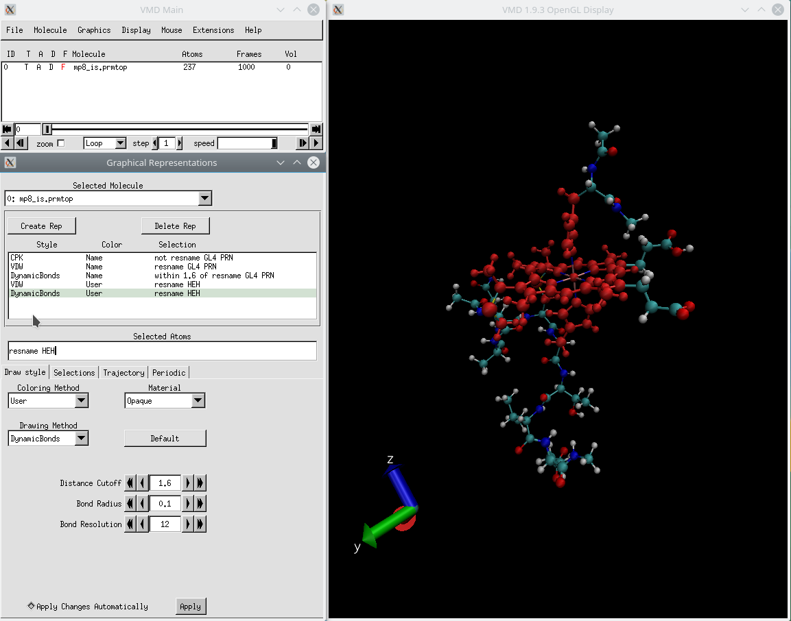
3. Change the Drawing Method in Graphical Representations console to CPK, and under Selected Atoms type: not resname GL4 PRN
4. Click the tab Create Rep, change the Drawing Method to VDW, reduce the Sphere Scale to 0.3, and under Selected Atoms type: resname GL4 PRN
5. Click the tab Create Rep, change the Drawing Method to Dynamic Bonds, reduce the Bond Radius to 0.1, and under Selected Atoms type: within 1.6 of resname GL4 PRN
6. Create one new replica for each of the last two replicas created (VDW and DynamicBonds)
7. On the last two replicas just created, change the Coloring Method to Trajectory→User→User, and under Selected Atoms type: resname HEH
8. In the Graphical Representations window, go to the Trajectory tab, and make sure to set the Color Scale Data Range from 0.0 to 100.0

This is how your final screen in VMD should look like:

---

Click here to go to Section 4

---

Click here to go back to Section 2

---

References

[1] Vinícius Wilian D. Cruzeiro, Marcos S. Amaral, and Adrian E. Roitberg, "Redox Potential Replica Exchange Molecular Dynamics at Constant pH in AMBER: Implementation and Validation", J. Chem. Phys., 149, 072338 (2018). DOI: https://doi.org/10.1063/1.5027379

[2] H.M. Marques, I. Cukrowski, and P.R. Vashi, "Co-ordination of weak field ligands by N-acetylmicroperoxidase-8 (NAcMP8), a ferric haempeptide from cytochrome c, and the influence of the axial ligand on the reduction potential of complexes of NAcMP8", J. Chem. Soc. Dalt. Trans., 8, 1335 (2000).

(Note: These tutorials are meant to provide illustrative examples of how to use the AMBER software suite to carry out simulations that can be run on a simple workstation in a reasonable period of time. They do not necessarily provide the optimal choice of parameters or methods for the particular application area.)
Copyright Vinícius Cruzeiro. 2018