


(Note: These tutorials are meant to provide
illustrative examples of how to use the AMBER software suite to carry out
simulations that can be run on a simple workstation in a reasonable period of
time. They do not necessarily provide the optimal choice of parameters or
methods for the particular application area.)
Copyright Vinícius Cruzeiro. 2018
Section 4: Running and analyzing production simulations at different pH and Redox Potential values
We will now see how we can run and analyze simulations at different values of pH and redox potential. This will allow us to make more accurate Eo and pKa predictions, and also to evaluate the pH-effect on Eo and the redox potential-effect on pKa values. For simplicity, we will only make calculations in implicit solvent here, however, the same procedure can be followed in explicit solvent.
Running the simulations
We now need to replicate the input file used in the production phase shown in Section 3 for different pH and redox potential values. This can be easily done by using a simple bash script that makes use of the sed Linux command. The first step is to change the value of solvph by PH and solve by REDOX in a reference input file. PH and REDOX are pointers to be replaced by the script with values of pH and redox potential. This is how the reference input file should look like:
| prod.implicit.mdin.ref |
|
Production Stage in Implicit Solvent &cntrl icnstph=1, ! Switch for constant pH (=1, implicit solvent) ntcnstph=5, ! Protonation state change attempt every ntcnstph steps solvph=PH, ! Solvent pH icnste=1, ! Switch for constant redox potential (=1, implicit solvent) ntcnste=5, ! Protonation state change attempt every ntcnste steps solve=REDOX, ! Solvent redox potential (in Volts) ntt=3, ! Temperature scaling (=3, Langevin dynamics) gamma_ln=10.0, ! Collision frequency of the Langevin dynamics in ps-1 ntc=2, ! SHAKE constraints (=2, hydrogen bond lengths constrained) ntf=2, ! Force evaluation (=2, hydrogen bond interactions omitted) ntb=0, ! Boundaries (=0, non-periodic) cut=1000.0, ! Cutoff dt=0.002, ! The time step in picoseconds nstlim=10000000, ! Number of MD steps to be performed ig=-1, ! Random seed (=-1, get a number from current date and time) ntwr=10000, ! Restart file written every ntwr steps ntwx=10000, ! Trajectory file written every ntwx steps ntpr=10000, ! The mdout and mdinfo files written every ntpr steps ioutfm=1, ! Trajectory file format (=1, Binary NetCDF) igb=2, ! GB model saltcon=0.1, ! Salt concentration irest=1, ! Flag to restart the simulation ntx=5, ! Initial condition (=5, coord. and veloc. read from the inpcrd file) / |
We show below the simple bash script cphemd_geninputs.sh that helps generating the input files. For simplicity, only 6 values of pH and 6 values of redox potential are being considered. However, the script can be easily modifed to cover more values.
| cphemd_geninputs.sh |
|
#!/bin/bash # Reference input file infile=prod.implicit.mdin.ref for PH in {5.0,5.5,6.0,6.5,7.0,7.5} do for REDOX in {-0.263,-0.233,-0.203,-0.173,-0.143,-0.113} do newfile=${infile%.ref}.pH_$PH.E_$REDOX cp $infile $newfile sed -i "s/PH/$PH/g" $newfile sed -i "s/REDOX/$REDOX/g" $newfile done done |
This script will generate 36 input files in the format prod.implicit.mdin.pH_*.E_* (note that the suffix .ref was removed).
We now need to execute the simulations. As the simulations are independent, they can be executed simultaneously in parallel to save time. In case you want to execute the simulations in serial, the following script can be used:
| cphemd_run.sh |
|
#!/bin/bash # Reference input file infile=prod.implicit.mdin.ref # Topology file prmfile=mp8_is.prmtop # Input rst7 file crdfile=mp8_is.equi.rst7 # CPIN file cpin=mp8_is.cpin # CEIN file cein=mp8_is.cein # Prefix for the output files prefix=mp8_is.prod for PH in {5.0,5.5,6.0,6.5,7.0,7.5} do for REDOX in {-0.263,-0.233,-0.203,-0.173,-0.143,-0.113} do newfile=${infile%.ref}.pH_$PH.E_$REDOX pmemd.cuda -O -i $newfile -p $prmfile -c $crdfile \ -x $prefix.nc.pH_$PH.E_$REDOX -inf $prefix.mdinfo.pH_$PH.E_$REDOX \ -o $prefix.mdout.pH_$PH.E_$REDOX -r $prefix.rst7.pH_$PH.E_$REDOX \ -cpin $cpin -cpout $prefix.cpout.pH_$PH.E_$REDOX \ -cprestrt $prefix.cprestrt.pH_$PH.E_$REDOX \ -cein $cein -ceout $prefix.ceout.pH_$PH.E_$REDOX \ -cerestrt $prefix.cerestrt.pH_$PH.E_$REDOX done done |
The following tar file contains the CPOUT and CEOUT files generated in the simulations: couts.tar.gz.
Analysing the simulations
Theoretical background
From the Hendersen-Hasselbalch equation we can devise an expression for the fraction of protonated species of a given pH-active residue:
f_{prot} = \frac 1 {1 + 10 ^ {n (pH - pK_a)}} [1]
where n is the Hill coefficient.
Equivalently, from the Nernst equation we can devise an expression for the fraction of reduced species of a given redox-active residue (see reference [1] for more information):
f_{red} = \frac 1 {1 + e ^ {n \frac{\nu F}{k_b T} (E - E^o)}} [2]
where n is the Hill coefficient, \nu is the number of electrons being reduced in the redox reaction, F is the Faraday constant, k_b is the Boltzmann constant, T is the temperature, and E is the redox potential.
Using fitpkaeo.py
The fitpkaeo.py AmberTool allows us to automatically get fitted values of pKa and Eo using equations 1 and 2. This is obtained by passing information from cphstats or cestats for multiple CPOUT or CEOUT files to fitpkaeo.py through pipe. fitpkaeo.py is able to even generate a graph containing the fractions from the simulations against the fitted curve.
For example, to fit the Eo value of residue HEH at pH 7.0 and generate the
graph, we can use the command:
for ceout in mp8_is.prod.ceout.pH_7.0.E_-0.*; do cestats -i mp8_is.cein $ceout; done
| fitpkaeo.py --graph --graph-path fracredu.png
This will generate the following output:
HEH 14: Eo = -0.202811 (+- 0.000296 ) V; Hill coefficient =
1.028 (+- 0.011 ); Temperature = 300.00 K
Graph generated to fracredu.png
and the following figure:
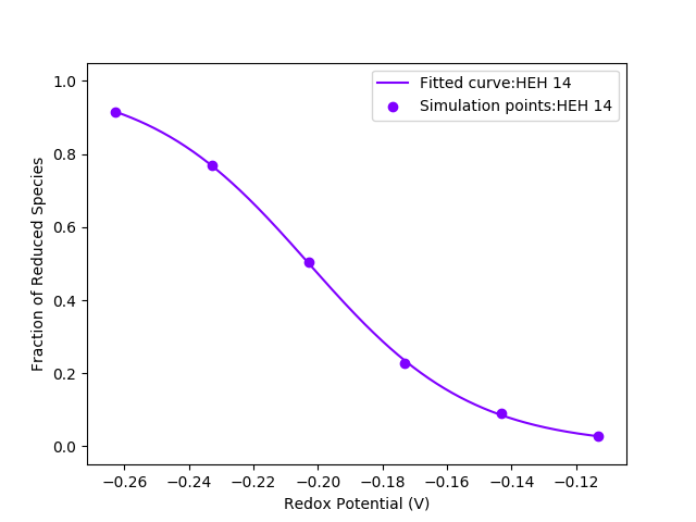
As can be seen, we successfully obtain a Eo value very close to our target value of -203 mV at pH 7.0. The values inside the parenthesis represent fitting errors of the properties shown. The low fitting errors are justified in the figure. As we can see, the fractions of reduced species obtained through the simulations for different redox potential values at pH 7.0 lie very well on top of the fitted curve.
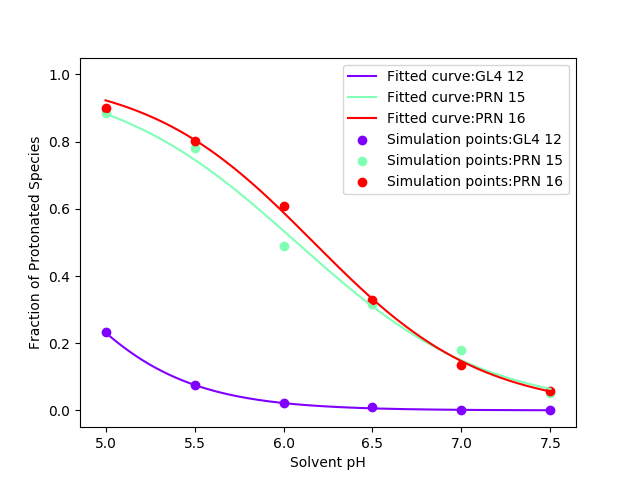
Let's now fit the pKa values of all pH-active residues at redox potential
-203 mV. We can do this with the following command, which also generates a graph:
for cpout in mp8_is.prod.cpout.pH_*.E_-0.203; do cphstats -i mp8_is.cpin $cpout; done
| fitpkaeo.py --graph --graph-path fracprot.png
This command will generate the following output:
GL4 12: pKa = 4.53952 (+- 0.00894 ) ; Hill coefficient = 1.130 (+- 0.017 )
PRN 15: pKa = 6.07351 (+- 0.04300 ) ; Hill coefficient = 0.817 (+- 0.063 )
PRN 16: pKa = 6.16959 (+- 0.01876 ) ; Hill coefficient = 0.921 (+- 0.034 )
Graph generated to fracprot.png
and the following figure:
pH-dependence of Eo predictions
We can use the following command to generate Eo fittings at different pH values:
for PH in {5.0,5.5,6.0,6.5,7.0,7.5}
do
echo pH: $PH
for ceout in mp8_is.prod.ceout.pH_$PH.E_*; do cestats -i mp8_is.cein $ceout; done
| fitpkaeo.py
done
This will generate the following output:
pH: 5.0
HEH 14: Eo = -0.186541 (+- 0.000713 ) V; Hill coefficient = 0.984 (+- 0.024 ); Temperature = 300.00 K
pH: 5.5
HEH 14: Eo = -0.189420 (+- 0.001411 ) V; Hill coefficient = 1.057 (+- 0.055 ); Temperature = 300.00 K
pH: 6.0
HEH 14: Eo = -0.198200 (+- 0.000624 ) V; Hill coefficient = 1.020 (+- 0.023 ); Temperature = 300.00 K
pH: 6.5
HEH 14: Eo = -0.199265 (+- 0.000638 ) V; Hill coefficient = 1.025 (+- 0.024 ); Temperature = 300.00 K
pH: 7.0
HEH 14: Eo = -0.202811 (+- 0.000296 ) V; Hill coefficient = 1.028 (+- 0.011 ); Temperature = 300.00 K
pH: 7.5
HEH 14: Eo = -0.205623 (+- 0.000310 ) V; Hill coefficient = 0.963 (+- 0.010 ); Temperature = 300.00 K
We can plot this data to obtain the Eo of HEH as a function of pH.
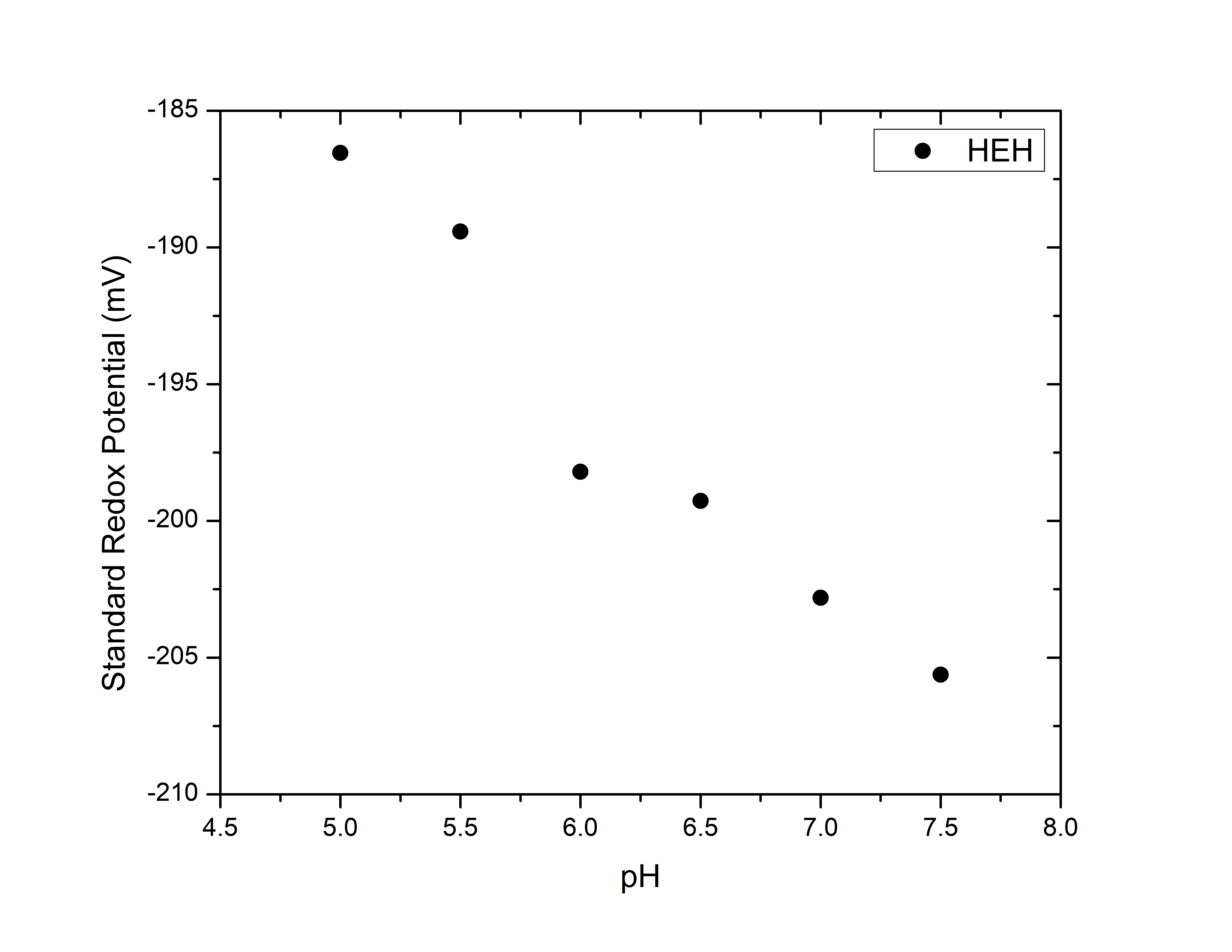
As discussed in reference [1], Eo should decrease with pH. As the figure shows, this behavior is correctly described by our simulations.
Redox potential-dependence of pKa predictions
The following command prints the fittings of the pKa values of all pH-active
residues for different redox potential values:
for REDOX in {-0.263,-0.233,-0.203,-0.173,-0.143,-0.113}
do
echo Redox Potential: $REDOX V
for cpout in mp8_is.prod.cpout.pH_*.E_$REDOX; do cphstats -i mp8_is.cpin $cpout; done
| fitpkaeo.py
done
This will generate the following output:
Redox Potential: -0.263 V
GL4 12: pKa = 4.71920 (+- 0.03529 ) ; Hill coefficient = 1.311 (+- 0.116 )
PRN 15: pKa = 6.18241 (+- 0.06711 ) ; Hill coefficient = 0.766 (+- 0.088 )
PRN 16: pKa = 6.15350 (+- 0.03770 ) ; Hill coefficient = 0.766 (+- 0.049 )
Redox Potential: -0.233 V
GL4 12: pKa = 4.76361 (+- 0.03594 ) ; Hill coefficient = 1.363 (+- 0.137 )
PRN 15: pKa = 6.09123 (+- 0.04907 ) ; Hill coefficient = 0.835 (+- 0.075 )
PRN 16: pKa = 6.25073 (+- 0.04109 ) ; Hill coefficient = 0.740 (+- 0.051 )
Redox Potential: -0.203 V
GL4 12: pKa = 4.53952 (+- 0.00894 ) ; Hill coefficient = 1.130 (+- 0.017 )
PRN 15: pKa = 6.07351 (+- 0.04300 ) ; Hill coefficient = 0.817 (+- 0.063 )
PRN 16: pKa = 6.16959 (+- 0.01876 ) ; Hill coefficient = 0.921 (+- 0.034 )
Redox Potential: -0.173 V
GL4 12: pKa = 4.37096 (+- 0.11188 ) ; Hill coefficient = 0.856 (+- 0.117 )
PRN 15: pKa = 5.96110 (+- 0.03184 ) ; Hill coefficient = 0.835 (+- 0.049 )
PRN 16: pKa = 6.11422 (+- 0.01552 ) ; Hill coefficient = 0.851 (+- 0.024 )
Redox Potential: -0.143 V
GL4 12: pKa = 4.18668 (+- 0.01406 ) ; Hill coefficient = 0.900 (+- 0.013 )
PRN 15: pKa = 5.97212 (+- 0.02218 ) ; Hill coefficient = 0.756 (+- 0.029 )
PRN 16: pKa = 6.07389 (+- 0.04610 ) ; Hill coefficient = 0.730 (+- 0.056 )
Redox Potential: -0.113 V
GL4 12: pKa = 3.94276 (+- 0.26421 ) ; Hill coefficient = 0.616 (+- 0.121 )
PRN 15: pKa = 6.00046 (+- 0.05143 ) ; Hill coefficient = 0.793 (+- 0.072 )
PRN 16: pKa = 6.13903 (+- 0.05881 ) ; Hill coefficient = 0.704 (+- 0.067 )
By plotting this data we obtain the pKa of each pH-active residue as a function
of redox potential.
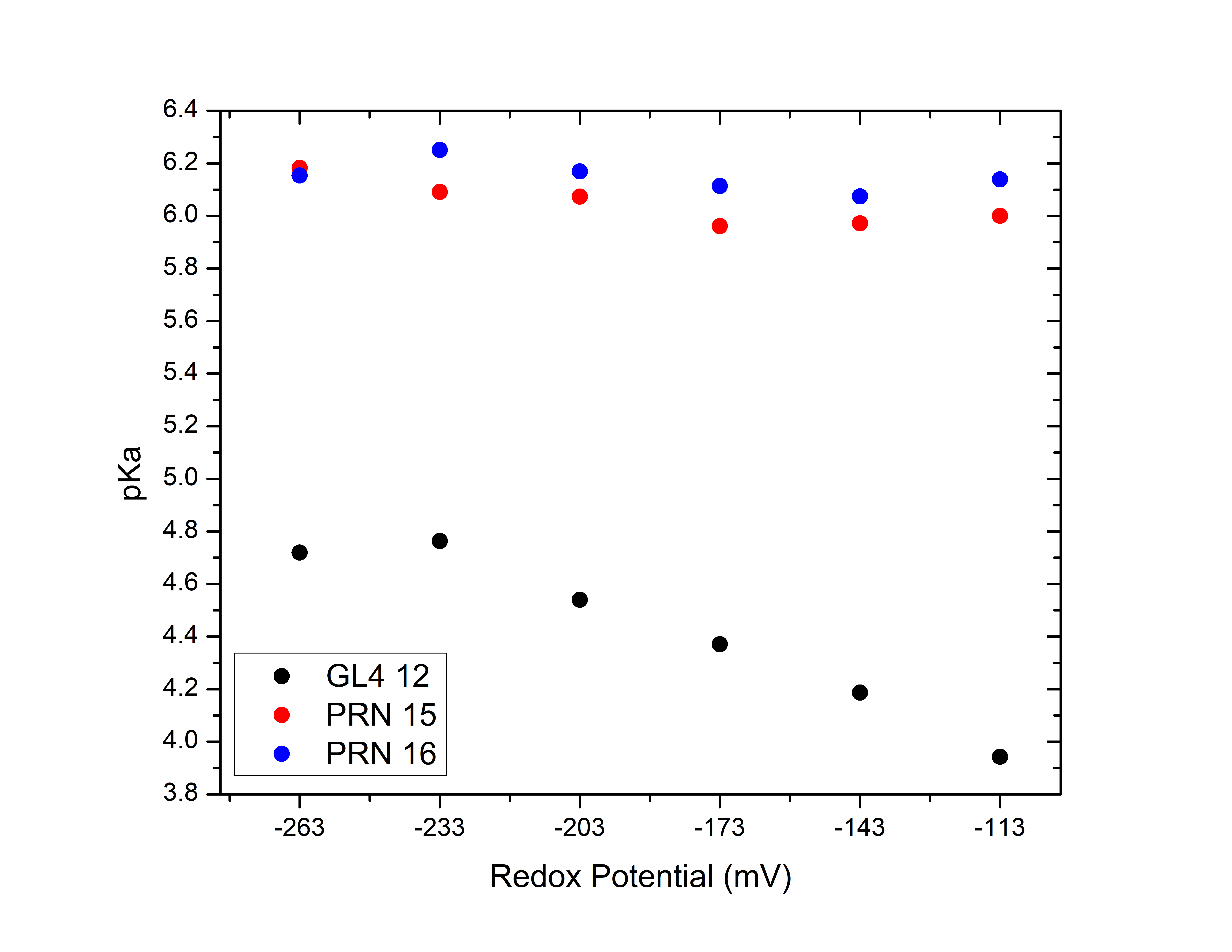
We see the pKa values decrease with increases in the redox potential, in agreement with the expectation (see reference [1]).
How can we increase convergence?
From the last two figures, it is clear that our results are still not converged. We would need to run longer to get a better convergence, or, as discussed in reference [1], make use of Redox Potential Replica Exchange MD (E-REMD) to obtain improved convergence. Reference [1] shows that E-REMD significantly improves sampling convergence in comparison to performing C(pH,E)MD only, thus without exchange attempts (as done in this section). The procedure to execute E-REMD in Amber is equivalent to running pH-REMD. Therefore, a nice pH-REMD tutorial written by Jason Swails that can be found here can be used as a reference. As opposed to the option "-rem 4" using in pH-REMD, in E-REMD we use "-rem 5". More information about E-REMD can also be found in Amber's manual.
The converged behavior of Eo versus pH and the pKa of each pH-active residue versus redox potential has been reported in reference [1]. There, simulations were performed longer, using E-REMD, and more values of pH and redox potential were considered.
Click here to go back to the Introduction
Click here to go back to Section 3
References
[1] Vinícius Wilian D. Cruzeiro, Marcos S. Amaral, and Adrian E. Roitberg, "Redox Potential Replica Exchange Molecular Dynamics at Constant pH in AMBER: Implementation and Validation", J. Chem. Phys., 149, 072338 (2018). DOI: https://doi.org/10.1063/1.5027379
(Note: These tutorials are meant to provide
illustrative examples of how to use the AMBER software suite to carry out
simulations that can be run on a simple workstation in a reasonable period of
time. They do not necessarily provide the optimal choice of parameters or
methods for the particular application area.)
Copyright Vinícius Cruzeiro. 2018