


Advanced Thermodynamic Integration (TI) Methods to Mutate a Ligand Bound to a Protein
by Shi ZhangaaDarrin York group, Rutgers University, Newark, NJ
Learning Outcomes
-Use Antechamber to derive force field parameters for ligands
Implementation Notes:
- DDBoost is a set of free energy tools developed by the York group, consisting of
FE_WorkflowFE_MDEngineFE_Toolkit
FE_MDEngineis in Amber22.FE_WorkflowandFE_Toolkitnot a part of Amber22, but files are compatible with Amber22, and available on the York gitlab page.
Introduction
This tutorial will guide you through calculating the relative binding free energies (ΔΔGbinding) between two ligands bound to the same protein. The system will be the human Thr160-phospho CDK2/cyclin A protein bound to two different inhibitors (NU6094 - PDBID: 1H1Q and NU6086 - PDBID: 1H1R).[1] This is a relatively conservative chemical change from H to Cl with only one “edge”. An edge is one alchemical transformation between two molecules. If you have more ligands or multiple function group changes between two ligands, you may need to perform multiple alchemical changes, in which case you should use MCS to define the softcore atoms for each edge.[2]
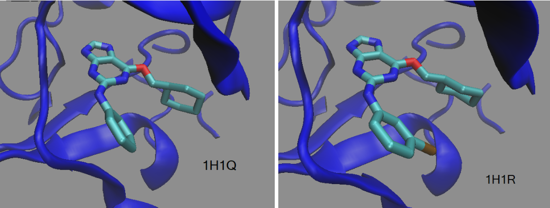 Figure 1. Ligands NU6094 (1H1Q) and NU6086 (1H1R) bound to the the human Thr160-phospho CDK2/cyclin A protein.
This tutorial assumes you know general Amber usage such as protein system setup, choices when relaxing a system and running production run molecular dynamics simulations. As well, it also assumes you know the fundamental issues surrounding free energy calculations. If you need more guidance, please see these tutorials:
- Building Protein Systems in Explicit Solvent
- Relaxation of Explicit Water Systems
- Running MD with pmemd
- Thermodynamic Integration using softcore potentials
Advanced TI Calculations
Free energies will be computed with thermodynamic integration (TI) with softcore potentials, a method used to ensure smooth free energy curves, as implemented in pmemd.cuda which runs on a GPU.[3] This implementation is a little more sophisticated than the standard TI. It will use FE_Workflow to create a number of inputs that will run GPU-driven Hamiltonian replica exchange molecular dynamics (HREMD) TI calculation method known as alchemical enhanced sampling (ACES)[4]
with recent flags available in Amber, including smoothstep softcore potentials and enhanced sampling methods.
In this tutorial, we’re going to use FE_Workflow, part of DDBoost, to set up the TI calculations, which will employ:
- a second-order smoothstep softcore potential.
- enhanced sampling
git_add_scfunctionalities. - Hamiltonian REMD with lambda TI as implemented in the ACES code.
Noteworthy TI Flags
Smoothstep Softcore Potentials
Many issues with linear interpolation between end states result in spurious energies and poor statistics (reviewed in ref [5] introduction). Concerted softcore potentials “soften” the Lennard-Jones and electrostatic interactions with increasing values of α and β parameters, respectively. The default values6 in Amber are
scalpha=0.5 and scbeta=12.
A second-order smoothstep softcore potential, SSC(2), was developed to alleviate some of the remaining energy issues, replacing the original softcore potentials and setting variables scalpha=0.2 and scbeta=50. The SSC(2) function with these values enable the free energy derivatives to vanish at the transformation endpoints and smooth adjustment of the λ-dependent terms in the potential.5
Enhanced Sampling for Softcore Ligand Energies
In theory, sampling will not affect the converged value of the ΔΔGbinding. However, in practice, for example when rotating a ligand from cis to trans, there may be steric hindrances in the protein binding pocket during calculation of the alchemical change. Enhanced sampling methods for softcore energy calculations have been developed to improve convergence.4
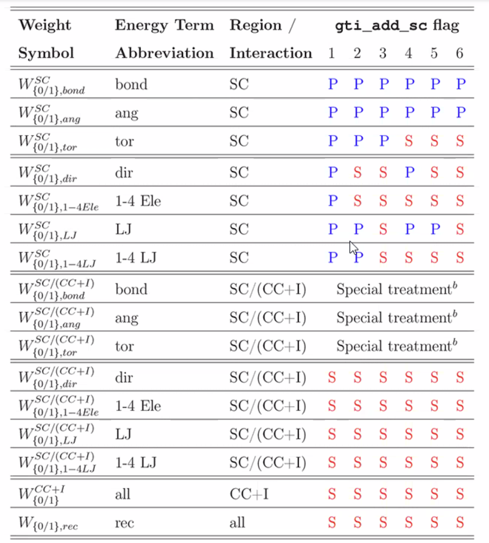
Figure 2. Softcore enhanced sampling flags in Amber. For more explanation, see text in ref 4.
If you think there is an issue with convergence, for instance, in your ΔΔGbinding calculation, you can scale interactions between the common core (e.g. pharmacophore) and your softcore region (the atoms that changed). Figure 2 lists gti_add_sc options, where S means that the interactions between the common core and softcore region will be scaled in lambda windows, but P means energies will stay constant for all lambda windows.
The default flag in Amber TI calculations is git_add_sc=1. Theoretically, you should obtain the same ΔΔGbinding with any of the 1-6 gti_add_sc values because G is a state function. However, in practice, the York group currently recommends gti_add_sc=5.
ACES Method on the Ligand
The alchemical enhanced sampling (ACES)[4] method is a Hamiltonian replica exchange molecular dynamics (HREMD) thermodynamic integration method that exchanges between lambda windows. This increases the sampling between neighboring lambda windows and should increase convergence of the calculated ΔΔGbinding between trials. This will require running on multiple GPUs on a single node (see below for an estimation of how many).
Reviews
More information is also available through these articles. [7, 8]
System Setup
Prepare the Protein•Ligand PDB Files – 1H1Q and 1H1R
1. Download the 1h1q structureRepeat Steps 1-3 for the 1H1R protein•ligand complex.
Derive Force Field Parameters for the Ligands with Antechamber
Force fields are specific for the molecule type. Ligands, usually organic molecules, are modelled in Amber with GAFF or some modification of this. For this tutorial, GAFF2 parameters will be derived with Antechamber. Each new ligand will require derivation of parameters with Antechamber unless they exist elsewhere in the literature.
4. Add hydrogens to the ligand using a tool such a VMD or Chimera X.- File
- New Molecule
- Resid 1298 = selection
- Select all
- +Hs
- Enlarge in VMD and look at Hs that are added.
- Delete extra Hs
- Make H’s planar if need be by selecting dihedral and then clicking “Force Planar”
- Make sure ligand picture looks chemically reasonable. Pay attention to the H’s that are added to the imidazole ring, to confirm whether they are added to the correct N atom.
- File Apply Changes to Parent, Yes
- Should see 1h1r_edited.pdb. Save it by File, Save Coordinates, selected atoms: “all”, file type - pdb.
- Click Save and name new file.
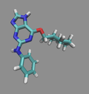 Figure 3. Ligand from 1H1Q (NU6094) after hydrogen atoms added with Molefacture.
Save changes
Using a text editor, rename the residue name (column 18 to 20) of the ligand from “2A6” to “LIG”
The residue name for all ligands should be “LIG” in order for DDBoost to recognize the ligands.
Using a text editor, copy the ligand to a new file named 1h1q_0.pdb. Simply copy-paste. Do not cut-paste because you don't want to remove it from the original protein•ligand complex coordinates.
mol2 file.
This run will use GAFF2 parameters and set net charge = 0 because LIG is a neutral ligand.
ndiis_attempts=700 ⇒ Forces antechamber to run enough times to generate a force field.
Here, {PDB} can be changed to "1h1q".
antechamber -i ${PDB}_0.pdb -fi pdb -o ${PDB}_0.mol2 -fo mol2 \
-at "gaff2" -pf y -an y -c 2 -nc 0 -rn LIG -ek "ndiis_attempts=700"
8. Run parmchk2 to get an frcmod file.
Here, {PDB} can be changed to "1h1q".
parmchk2 -i ${PDB}_0.mol2 -o ${PDB}_0.frcmod -f mol2 -s 1
9. Run tleap to generate an lib file.
Here, {PDB} can be changed to "1h1q".
tleap commands
loadamberparams ${PDB}_0.frcmod
LIG = loadmol2 ${PDB}_0.mol2
saveoff LIG ${PDB}_0.lib
quit
10. Repeat step 4-9 for other ligands.
For example, in this case, you want to repeat steps 4-9 for 1H1R where H is instead Cl.
- 1h1q.pdb
- 1h1q_0.frcmod
- 1h1q_0.lib
- 1h1q_0.mol2
- 1h1q_0.pdb
- 1h1r.pdb
- 1h1r_0.frcmod
- 1h1r_0.lib
- 1h1r_0.mol2
- 1h1r_0.pdb
Sample Files
All files required for intial setup are provided here. This includes:
***Note that you will need to make sure that the residue name for each ligand should be “LIG” in BOTH .pdb files and BOTH.lib files in order for DDBoost to recognize the ligands.
Simulation Setup
In this tutorial, we’re going to use FE_Workflow, part of DDBoost, to set up the TI calculations, which will employ:
- a second-order smoothstep softcore potential.
- enhanced sampling
git_add_scfunctionalities. - Hamiltonian REMD with lambda TI as implemented in the ACES code.
Setup directories and input file for FE_Workflow
FE_Workflow uses the input file to specify parameters. It assumes the following:
- A single place to put all the pdb files and frcmod files.
- Use the
inputfile to control different steps of the TI calculation (ex: setup or analysis; in this first case setup).
- Make a folder called
ti. - In the
tifolder, make two folders, one calledrbfeand another calledinitial. -
In the
initialfolder, make a subfolder for the protein. For example, call itCDK2. - Place all the frcmod files and pdb files from the System Setup into this folder (
initial/CDK2).
FE_Workflow will read in files found in initial/CDK2 and put results in the rbfe folder. In the rbfe folder, FE_Workflow will also make folders for each trial and lambda window, and then place TI input files, scripts, results in the correct folders. Figure 4 contains a list of files and/or folders the user needs to make (blue) and the ones the FE_Workflow will make (green).
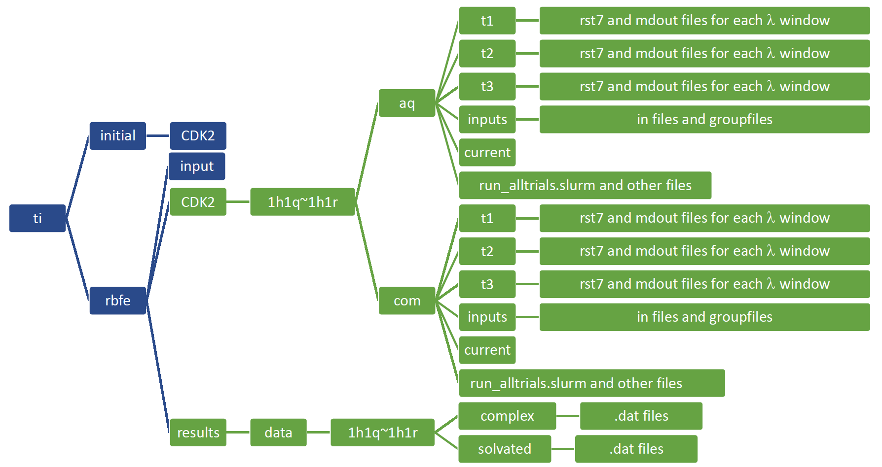
Figure 4. File setup for FE_Workflow.
- Either download the
inputfile or copy it from xxxx. - Place the
inputfile in yourtifolder. - Edit the input file. The user will need to specify the following flags:
For this tutorial, we are going to use the ff14SB protein force field and gaff2 for ligand force field. The water model is set to tip4pew and the buffer size is 16 Å for complex system and 20 Å for solution system. We'll use tleap to add a water box and ions.
FE_Workflow will build an extensive set of input and scripting files necessary to run a robust equilbiration, including solvent relaxation, heating and production run for 2 ns at each lambda step. This is all contained in the run_alltrials.slurm file. Default values are used in FE_Workflow. If you want to modify the relaxation, heating or production runs, you can manually modify the md.in files for each step after FE_Workflow has made all the files.
In this tutorial, we are running 11 lambda windows in parallel for 20 steps. After 20 steps, an exhange is attempted with a neighboring lambda window. At the exchange step, will try to exchange if successful, will run for another 20 steps and then another exchange. The flag numexchg controls how many exchanges will be attempted and nstlim specifies how many steps between exchange attempts.
| Flag | Example Setting | What happens |
| Path_to_input | initial | sets the path of the setup (this has to exist already) |
| system | initial/CDK2 | sets the path of the protein (this has to exist already) |
| stage | setup | sets if this is setup or analysis |
| translist | 1h1q~1h1r | sets the name of the folder for the transformation. FE_Workflow will make this folder |
There is a detailed explanation for the flags inside the sample input file and Amber Reference Manual. For instance, under:
#######################################################################
# 1. NAME OF SYSTEM, INPUT STRUCTURES, and TYPE OF CALCULATION
#######################################################################
and
# List of desired transformations or edgesThere are directions for specifying the names of the tranformations.
# For example, RBFE or RSFE calculations should have a list
# in which each entry consists of two molnames separated by the
# character "~". Initial structure/parameter files of these
# molnames should be provided in /
# For RBFE calculations, the PDB file of protein-ligand complex
# and mol2,lib,frcmod files of ligand are expected.
# For RSFE calculations, mol2,lib,frcmod files of ligand are expected.
# example,
# translist=(1h1q~1h1r 1h1q~1h1s)
#
# For ASFE calculations, "translist" should contain a list of
# molnames.
# mol2,lib,frcmod files of these molnames are expected in
# /
# example,
# translist=(mobley_1527293 mobley_3034976)
#translist=(1h1q~1h1r 1h1r~1h1s 1h1s~1oiu 1oiu~1h1q 1h1r~1oiu 1h1s~1h1q)
Run FE_Workflow
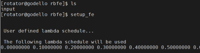
13. Go to the folder withinput, type the command
setup_fe
Workflow should begin to generate the files for you.
In your transformation folder, FE_Workflow will make a set of folders, one for the ligand solvated in water (aq) and for the protein•ligand complex (com). It will copy over needed .parm7 and .rst7 files, as well as make .sh and slurm files.
You will find simulation topology, coordinate, md input and slurm files under CDK2/1h1q~1h1r/aq and com folders respectively (see Figure 4). Files for the set of the transformation 1h1q to 1h1r are provided for your reference.
In the beginning, the trial folders (t1, t2 and t3) only contain .rst7 files for end states (0 and 1). Later it will later write .mdout, .nc files as well as .rst7 files for propagated lambda windows from equilibration.
Running the TI Calculation
14. The user should edit the slurm script to customize the number of GPUs requested.GPU Usage
This TI implementation uses ACES, a replica exchange method, that requires multiple GPUs to run simultaneoulsy.
You might ask how many GPUs you need. You do not need the same number of GPUs as replicas. The number of replicas per GPU is determined by the GPU memory size. If your GPU has a lot of memory (ex: 32 GB), you can put 20 replicas on 1 GPU. A typical system with 100,000 atoms, will take 1 GB GPU memory. Modern GPUs typically have 8 GB memory. Therefore, about 8 replicas can go on 1 GPU simultaneously. The code will of course go faster if you have more GPUs. The slurm script will automatically distribute the replicas to the specified number of GPUs available. For instance, if you tell slurm to grab 2 GPUs, will put 5 in 1 GPU and 6 replicas in the other. If you have 4 GPUs, it will distribute the 11 replicas evenly. NOTE: All the GPUs should be on the same node. If you are using multiple nodes, it will slow down the exchange attempt due to I/O communication issues.
15. Submit the slurm script.
Now transfer the files to any HPC where FE-MDEngine is installed. Confirm the “#SBATCH --” lines are set appropriately. Submit the slurm script and wait for the simulations to finish. The simulation will go through minimization, equilibration and production stages. Each step will generate the output file and coordinate. Here is an example production run input.
&cntrl
imin            = 0
nstlim          = 20
numexchg        = 100000
dt              = 0.001
irest           = 0
ntx             = 1
ntxo            = 1
ntc             = 1
ntf             = 1
ntwx            = 10000
ntwr            = 5000
ntpr            = 1000
cut             = 10
iwrap           = 1

ntb             = 2
temp0           = 298.
ntt             = 3
gamma_ln        = 2.
tautp           = 1
ntp             = 1
barostat        = 2
pres0           = 1.01325
taup            = 5.0

ifsc            = 1
icfe            = 1

ifmbar          = 1
bar_intervall   = 1
mbar_states     = 11
mbar_lambda(1)     = 0.00000000
mbar_lambda(2)     = 0.10000000
mbar_lambda(3)     = 0.20000000
mbar_lambda(4)     = 0.30000000
mbar_lambda(5)     = 0.40000000
mbar_lambda(6)     = 0.50000000
mbar_lambda(7)     = 0.60000000
mbar_lambda(8)     = 0.70000000
mbar_lambda(9)     = 0.80000000
mbar_lambda(10)     = 0.90000000
mbar_lambda(11)     = 1.00000000

noshakemask     = '@1-90'

clambda         = 1.00000000
timask1         = '@1-45'
timask2         = '@46-90'
crgmask         = ""
scmask1         = '@41'
scmask2         = '@90'
scalpha         = 0.5
scbeta          = 1.0

gti_cut         = 1
gti_output      = 1
gti_add_sc      = 5
gti_scale_beta  = 1
gti_cut_sc_on   = 8
gti_cut_sc_off  = 10
gti_lam_sch     = 1
gti_ele_sc      = 1
gti_vdw_sc      = 1
gti_cut_sc      = 2
gti_ele_exp     = 2
gti_vdw_exp     = 2

gremd_acyc      = 1
/
&ewald
/
Analysis of the Simulation
This tutorial uses FE_Toolkit to analyze the data automatically.
If simulations finish without errors, you will find a series of *ti.mdout files in the t1/ folder. For the free energy results, we will extract energy values from these *ti.mdout files.
Look at the trajectories of the endstates in VMD
If you want to take a close look at the conformation or the structure of the ligand, load in VMD the unisc.parm7 and 0.00000000_ti.nc for real state ligand 1h1q (resid :1), 1.00000000_ti.nc for real state ligand 1h1r (resid :2).
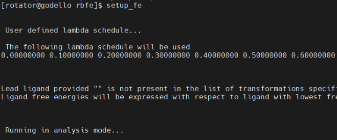
Perform Analysis
setup_fe
Essentially, the analysis uses the graphmbar program inside the FE-Toolkit, and there are more advanced options for different features you may want to explore. An example of graphmbar is provided in the fe-toolkit/src/graphmbar-0.9/examples/stx. A general usage is consisted of three steps:
python3 ./gmbar.py -f ExptData.txt -t 1 2 3 -c > graphmbar.inp
OMP_NUM_THREADS=1 mpirun -n 6 graphmbar_mpi --nboot=200 --fc=10.\
               --guess=2 graphmbar.inp > graphmbar.out
python3 ./gmbar.py -f ExptData.txt -t 1 2 3 \
         -a graphmbar.out > graphmbar.txt
The FE-Workflow serves as an interface to connect graphmbar and pass some variables for analysis.
The experimental value to the binding free energy is not passed to the analysis mode in this example, but you can always apply the experimental restraints by providing a file consisting of two column, first is the names of the complex, second the experimental value in unit of kcal/mol. Let’s look at the graphmbar.txt file. Since we only have two nodes, no cycle is detected.
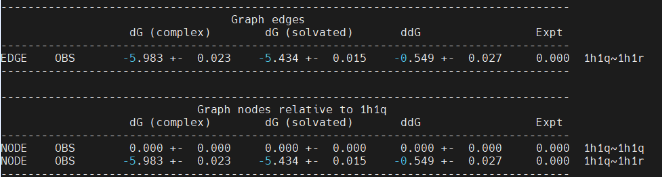
On the last line, it generates the relative binding free energy from 1h1q to 1h1r based on our one trial simulation. The ddG value is -0.549 kcal/mol.
References
- Davies, T. G., Bentley, J., Arris, C. E., Boyle, F. T., Curtin, N. J., Endicott, J. A., Gibson, A. E., Golding, B. T., Griffin, R. J., Hardcastle, I. R., Jewsbury, P., Johnson, L. N., Mesguiche, V., Newell, D. R., Noble, M. E. M., Tucker, J. A., Wang, L.,and Whitfield, H. J. Nature Structural and Molecular Biology, 2002, 9, 745-749.
- Cao, Y., Jiang, T., and Girke, T. A maximum common substructure-based algorithm for searching and predicting drug-like compounds. Bioinformatics, 2008, 24, i366–i374.
- Lee, T. S., Cerutti, D. S., Mermelstein, D., Lin, C., LeGrand, S., Giese, T.J., Roitberg, A., Case, D. A., Walker, R. C., and York, D. M. GPU-Accelerated Molecular Dynamics and Free Energy Methods in Amber18: Performance Enhancements and New Features. Journal of Chemical Information and Modeling, 2018, 58, 2043-2050.
- Lee, T. S., Tsai, H. C., Ganguly, A., and York, D. M. ACES: Optimized Alchemically Enhanced Sampling. Journal of Chemical Theory and Computation, 2023, 19, 472-487.
- Steinbrecher, T.; Joung, I.; Case, D. A. Soft-core potentials in thermodynamic integration: Comparing one- and two-step transformations J. Comput. Chem., 2011, 32, 3253– 3263.
- Lee, T.S., Lin, Z., Allen, B.K., Lin, C., Radak, B.K., Tao, Y., Tsai, H.-C., Sherman, W. and York, D.M. Improved Alchemical Free Energy Calculations with Optimized Smoothstep Softcore Potentials J. Chem. Theory Comput., 2020, 16, 5512–5525.
- Tsai, H. C., Lee, T. S., Ganguly, A., Giese, T. J., Ebert, M. C., Labute, P., Merz Jr., K. M., and York, D. M. AMBER Free Energy Tools: A New Framework for the Design of Optimized Alchemical Transformation Pathways. Journal of Chemical Theory and Computation, 2023, 19, 640-658.
- Ganguly, A., Tsai, H. C., Pendás-Fernández, M., Lee, T. S., Giese, T. J., and York, D. M. AMBER Drug Discovery Boost Tools: Automated Workflow for Production Free-Energy Simulation Setup and Analysis (ProFESSA). Journal of Chemical Information and Modeling, 2022, 62, 6069-6083.