


Relaxation of Explicit Water Systems
Learning Outcomes
- Understand the principles of relaxing a system solvated with explicit solvent
- Understand the difference between relaxation and equilibration
- Create stable systems containing explicit solvent
Process
1. Minimize the added water and ions
2. Heat up the system from 100 K under constant V
3. Relax under constant P
4. Lower the restraints on the system
5. Minimize the system with backbone restraints
6. Relax under constant pressure with backbone restraints
7. Reduce backbone restraints
8. Continue reducing backbone restraints
9. Run with no backbone restraints
10. Input Files and Script
•Run script
11. Checking Relaxation
Troubleshooting
Conclusion and Next Steps
Other Tutorials with Relaxation
Background
Explicit Solvent
Explicit solvent models include actual solvent atoms such as water molecule H and O. There are several explicit water models, such as TIP3P and OPC. Explicit water models should be matched with the solute force field and the ion model. For instance, ff14SB for proteins includes empirical corrections for using the TIP3P water model. For more information, please see the Amber Force Fields page and read Section 3.5 of the Amber Reference Manual.
This tutorial guides you through minimization and relaxation of systems with explicit solvent.
Note: There are two options for modeling solvents in simulations known as explicit or implicit solvent. Choosing between them are important decisions for an actual research project that we will not cover within this tutorial. To learn more about relaxing implicit solvent simulations, please consult this tutorial.
Relaxation
Formerly referred to as equilibration, relaxation aims to create stable systems. This consists of a series of steps involving minimization, heating up the system to a target temperature and tapering off restraints on the solute. Equilibration is no longer the preferred term, as it implies the system has definitively converged to a thermodynamically stable ensemble. Relaxation instead indicates the atoms in the system have been relaxed relative to one another's position. Relaxation is required to adapt the system from the initial model (e.g. crystal cell, cold, no hydrogens or water, etc. to a room temperature solution with all atoms). Even if the force field were perfect this needs to be done carefully and gradually to avoid having some drastic change happen that could be hard to fix later in production run molecular dynamics simluations.
MinimizationWhen the water molecules were added in leap, the box was added as the original water box containing only water molecules. For instance, the water molecules may behave differently when in the presence of a charged solute molecule. The first step in creating a stable system is to reduce bad contacts through the use of energy minimization. If we start molecular dynamics with these bad contacts, the energy in that region will be unrealistically high and as a result can crash the simulation, melt part of the structure, or cause the trajectory to proceed in an unrealistic direction. Minimization moves the atoms based on the forces and tries to find the closest structure that is at an energy minimum.
When performing minimization, the value imin is set to 1. In this tutorial, step 1 (1min.in) and step 5 (5min.in) are minimization steps. Options for minimzation are: sander, sander.MPI or pmemd.
This process involves increasing the temperature of the system to a target temperature while also decreasing the restraints on aspects of the system, which are performed under conditions of constant pressure and/or constant volume.
In step 2 (2mdheat.in), step 3 (3md.in), step 4 (4md.in), step 6 (6md.in), step 7 (7md.in), step 8 (8md.in), and step 9 (9md.in) run MD under various conditions. We use pmemd.cuda to perform MD. If you don't have pmemd.cuda, you can use pmemd, pmemd.MPI and/or sander but they will run slower than the GPU-enabled pmemd.
Process
In this tutorial, we will be using the human RAMP1 extracellular domain (PDBID: 2YX8) in an explicit solvent system containing the OPC water model. Please consult Tutorial 1.4. Building Protein Systems in Explicit Solvent if you would like to generate the starting files by yourself.
The starting files for this tutorial can be found here:
Input files and scripts for this tutorial are available here.
1. Minimize the added water and ions
The water molecules added with Leap are in positions optimized for water-water interactions. The positions do not take into account the presence of the solute or ions. This input minimizes the energy of water and ions. Everything else in the system is restrained.
1min.in
minimization of solvent
 &cntrl
  imin = 1, maxcyc = 1000,
  ncyc = 20, ntx = 1,
  ntwe = 0, ntwr = 500, ntpr = 50,
  ntc = 2, ntf = 2, ntb = 1, ntp = 0,
  cut = 10.0,
  ntr=1, restraintmask = ':1-81',
  restraint_wt = 100.,
  ioutfm=1, ntxo=2,
 /
Key settings (all others default as listed in the manual):
imin = 1       This run is a minimization run.
maxcyc = 1000  The maximum amount of minimization cycles is 1000.
ncyc = 20      The first 20 cycles will utilize the steepest descent
                  algorithm before shifting to the conjugate gradient
                  algorithm for the remaining cycles.
ntx = 1        The coordinates but not velocities are read formatted
                  from the coordinate file provided.
ntwe = 0       No mden files are written.
ntwr = 500     The amount of steps in which "restrt" files are written.
ntpr = 50      The amount of steps in which "mdout" and "mdinfo" files
                  are written.
ntc = 2        Bonds involving H are constrained.
ntf = 2        Bonds involving H are omitted from force evaluation.
ntb = 1        There is constant volume.
ntp = 0        There is no pressure scaling.
cut = 10.0     The non-bonded cutoff is 10.0 Angstroms.
ntr = 1        Use restraints.
restraintmask = ':1-81'  Restrain the solute - protein (res 1-81).
restraint_wt = 100  Positional restraint is 100 kcal/mol*Ang^-2.
ioutfm = 1     The format of the coordinate and velocity trajectory
                 files written as binary NetCDF.
ntxo=2         The "restrt" file format is NetCDF.
2. Heat up the system from 100 K under constant volume
This first step of relaxation will start the system from a low temperature of 100 K and gradually heat up to 298 K over 1 nanosecond of simulation time at a constant volume.
The heating occurs from the beginning in which the atoms are given random velocities that result in a Maxwell-Boltzmann distribution of velocities at the target temperature temp0. We start lower than the desired temperature and then slowly heat to our desired temperature. This helps adjust the system slowly and keeps it stable. However, when choosing your initial temperature, don't start the system at 0 K. This is because it will require a lot of heating and it can also make the system unstable.
 &cntrl
  imin = 0, nstlim = 1000000, dt = 0.001,
  irest = 0, ntx = 1, ig = -1,
  tempi = 100.0, temp0 = 298.0,
  ntc = 2, ntf = 2, tol = 0.00001,
  ntwx = 10000, ntwe = 0, ntwr = 1000, ntpr = 1000,
  cut = 8.0, iwrap = 0,
  ntt =3, gamma_ln=1., ntb = 1, ntp = 0,
  nscm = 0,
  ntr=1, restraintmask=':1-81', restraint_wt=100.0
  nmropt=1,
  ioutfm=1, ntxo=2,
 /
&wt TYPE="TEMP0", istep1=0, istep2=1000000, value1=100., value2=298., /
&wt TYPE="END", /
Key settings:
imin = 0          This is not a minimization run.
nstlim = 1000000  There will be 1000000 MD-steps.
dt = 0.001        There is a time step of 1 femtosecond.
irest = 0         The simulation will not be restarted.
ntx = 1           The coordinates but not velocities are read
                    formatted from the coordinate file provided.
ig = -1           The random seed number is based on the current
                    date and time of the run.
tempi = 100.0     The initial temperature is 100.0 K.
temp0 = 298.0     The reference temperature is set to 298.0 K
ntc = 2           Bonds involving H are constrained.
ntf = 2           Bonds involving H are omitted from force evaluation.
tol = 0.00001     The error of tolerance is 0.00001 Angstroms.
ntwx = 10000      The coordinates are written to a mdcrd file 10000 times.
ntwe = 0          No mden files are written.
ntwr = 1000       Number of steps in which "restrt" files are written.
ntpr = 1000       Number of steps in which "mdout" and "mdinfo"
                    files are written.
cut = 8.0         The non-bonded cutoff is 8.0 Angstroms.
iwrap = 0         No wrapping is performed.
ntt = 3           Langevin thermostat for temperature control is set.
gamma_ln=1.       The collision frequency gamma is set to 1 picosecond.
ntb = 1           There is constant volume.
ntp = 0           There is no pressure scaling.
nscm = 0          There is no removal of center of mass motion.
ntr=1             Atoms which are restrained within the simulation.
restraintmask = ':1-81' Restrain solute (as in 1min.in).
restraint_wt = 100  Positional restraint is 100 kcal/mol*Ang^-2.
nmropt=1          NMR restraints and weight changes will be read.
ioutfm = 1        The format of the coordinate and velocity trajectory
                    files written as binary NetCDF.
ntxo=2            The "restrt" file format is NetCDF.
The &wt section is setting parameters for varying conditions, changing during MD run. Each parameter is specified by a separate &wt namelist block, ending with &wt type=’END’.
TYPE="TEMP0"                  The target T will vary.
istep1=0, istep2=1000000      Change in T will occur in 1000000 increments.
value1=100., value2=298.      T begins at 100.0 K and increases to 298.0 K.
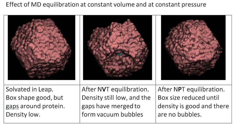
3. Relax the system at a constant pressure
This second step of relaxation will maintain the system from at 298 K over 1 nanosecond of simulation time at a constant pressure, allowing the box density to relax.
Question: Why don't we start with constant pressure right from the beginning?
Answer: If we ran constant pressure and there was a region with very high energy, it could cause high pressure, and the box would expand as a result. Our approach is to keep the box fixed at a constant volume while we correct any really bad problems, and then in the next steps we start using constant pressure to relax the box size and density.
 &cntrl
  imin = 0, nstlim = 1000000, dt = 0.001,
  irest = 1, ntx = 5, ig = -1,
  temp0 = 298.0,
  ntc = 2, ntf = 2, tol = 0.00001,
  ntwx = 10000, ntwe = 0, ntwr = 1000, ntpr = 1000,
  cut = 8.0, iwrap = 0,
  ntt =3, gamma_ln=1.0, ntb = 2, ntp = 1, barostat = 2,
  nscm = 0,
  ntr=1, restraintmask=':1-81', restraint_wt=100.
  ioutfm=1, ntxo=2,
 /
Key settings:
imin = 0          This run is not a minimization run.
nstlim = 1000000  There will be 1000000 MD-steps.
dt = 0.001        There is a time step of 1 fs.
irest = 1         Restart the simulation from previously
                    saved restart files.
ntx = 5           The coordinates and velocities are
                    read into the run.
ig = -1           The random seed number is based on the
                    current date and time of the run.
temp0 = 298.0     The reference temperature is set to 298 K.
ntwx = 10000      The coordinates are written to a mdcrd file 10000 times.
cut = 8.0         The non-bonded cutoff is 8.0 Angstroms.
ntt = 3           Langevin thermostat for temperature control is set.
gamma_ln=1.       The collision frequency gamma is set to 1 picosecond.
ntb = 2           Constant pressure.
ntp = 1           Use isotropic position scaling.
barostat = 2      Use the Monte Carlo barostat.
nscm = 0          No removal of center of mass motion.
ntr=1             Atoms which are restrained within the simulation.
restraintmask = ':1-81' Restrain solute (as in previous steps).
restraint_wt = 100  Positional restraint is 100 kcal/mol*Ang^-2 (same as above).
nmropt=1          NMR restraints and weight changes will be read.
ioutfm = 1        The format of the coordinate and velocity trajectory
                    files written as binary NetCDF.
ntxo=2            The "restrt" file format is NetCDF.
4. Lower the restraints on the system
This third step of MD will run MD over 1 ns at constant pressure and 298 K with a smaller restraint of 10 kcal/mol•Å2.
4md.in
 &cntrl
  imin = 0, nstlim = 1000000, dt = 0.001,
  irest = 1, ntx = 5, ig = -1,
  temp0 = 298.0,
  ntc = 2, ntf = 2, tol = 0.00001,
  ntwx = 10000, ntwe = 0, ntwr = 1000, ntpr = 1000,
  cut = 8.0, iwrap = 0,
  ntt =3,  gamma_ln=1.0, ntb = 2, ntp = 1,
  nscm = 0, barostat = 2,
  ntr=1, restraintmask=':1-81', restraint_wt=10.
  ioutfm=1, ntxo=2,
 /
Settings are all the same as 3md.in except the restraint_wt = 10.
5. Minimize the system with restraints just on the backbone of the molecule
Minimization of the system with restraints only on the backbone of the protein. In earlier runs, all atoms of the protein were restrainted. Now it's just the backbone atoms.
Note: The atoms to be restrained in this step will vary depending on your system. If you have molecules other than a protein,such as DNA or RNA, the "backbone" atom names will differ.
5min.in
Minimization of everything excluding backbone
 &cntrl
  imin = 1, maxcyc = 1000,
  ncyc = 30, ntx = 1,
  ntwe = 0, ntwr = 500, ntpr = 50,
  ntc = 2, ntf = 2, ntb = 1, ntp = 0,
  cut = 8.0,
  ntr=1, restraintmask="@CA,N,C", restraint_wt=10.
  ioutfm=1, ntxo=2,
 /
Key settings:
imin = 1        This run is a minimization run.
maxcyc = 1000   The maximum amount of minimization cycles is 1000.
ncyc = 30       The first 30 cycles will utilize the steepest descent
                   algorithm before shifting to the conjugate gradient
                   algorithm for the remaining cycles.
ntx = 1         The coordinates but not velocities are read formatted
                   from the coordinate file provided.
ntwe = 0        No mden files are written.
ntwr = 500      Number of steps "restrt" files are written.
ntpr = 50       Number steps in which "mdout" and "mdinfo" files are written.
ntr = 1         Use restraints
restraintmask = "@CA,N,C"  This string specifies that alpha C, N, and
                   carbons are all restrained.
restraint_wt = 10  Weight of the positional restraint is 10 kcal/mol*Ang^-2.
6. Relax system at a constant pressure with backbone restraints
Relaxation over 1 ns of simulation time at a constant pressure with backbone restraints set to 10 kcal/mol•Å2.
6md.in
 &cntrl
  imin = 0, nstlim = 1000000, dt = 0.001,
  irest = 0, ntx = 1, ig = -1,
  tempi = 298.0, temp0 = 298.0,
  ntc = 2, ntf = 2, tol = 0.00001,
  ntwx = 10000, ntwe = 0, ntwr = 1000, ntpr = 1000,
  cut = 8.0, iwrap = 0,
  ntt =3, gamma_ln=1.0, ntb = 2, ntp = 1,
  nscm = 0, barostat = 2,
  ntr=1, restraintmask="@CA,N,C", restraint_wt=10.
  ioutfm=1, ntxo=2,
 /
Key settings:
Settings are the same as 4md.in except:
restraintmask = "@CA,N,C"  This string specifies that alpha C, N, and
                   carbons are all restrained.
restraint_wt = 10  Weight of the positional restraint is 10 kcal/mol*Ang^-2.
7. Reduce the backbone restraint force
Relaxation for 1 ns of simulation time at a constant pressure with restraints on the backbone lowered to 1 kcal/mol•Å2.
7md.in
 &cntrl
  imin = 0, nstlim = 1000000, dt = 0.001,
  irest = 1, ntx = 5, ig = -1,
  temp0 = 298.0,
  ntc = 2, ntf = 2, tol = 0.00001,
  ntwx = 10000, ntwe = 0, ntwr = 1000, ntpr = 1000,
  cut = 8.0, iwrap = 0,
  ntt =3, gamma_ln=1.0, ntb = 2, ntp = 1,
  nscm = 0, barostat = 2,
  ntr=1, restraintmask="@CA,N,C", restraint_wt=1.
  ioutfm=1, ntxo=2,
 /
Key settings:
Settings are the same as 6md.in except:
restraint_wt = 1 Weight of the positional restraint is 1 kcal/mol*Ang^-2.
8. Continue to reduce the backbone restraint force.
Relaxation for 1 ns of simulation time at a constant pressure with restraints on the backbone lowered to 0.1 kcal/mol•Å2.
8md.in
 &cntrl
  imin = 0, nstlim = 1000000, dt = 0.001,
  irest = 1, ntx = 5, ig = -1,
  temp0 = 298.0,
  ntc = 2, ntf = 2, tol = 0.00001,
  ntwx = 10000, ntwe = 0, ntwr = 1000, ntpr = 1000,
  cut = 8.0, iwrap = 0,
  ntt =3, gamma_ln=1.0, ntb = 2, ntp = 1,
  nscm = 0, barostat = 2,
  ntr=1, restraintmask="@CA,N,C", restraint_wt=0.1
  ioutfm=1, ntxo=2,
 /
Key settings:
Settings are the same as 7md.in except:
restraint_wt = 0.1 Weight of the positional restraint is 0.1 kcal/mol*Ang^-2.
9. Relax the system with no restraints
This last step of relaxation removes the restraints on the backbone,simulates 1 ns of simulation time at a constant pressure.
9md.in&cntrl imin = 0, nstlim = 1000000, dt = 0.001, irest = 1, ntx = 5, ig = -1, temp0 = 298.0, ntc = 2, ntf = 2, tol = 0.00001, ntwx = 10000, ntwe = 0, ntwr = 1000, ntpr = 1000, cut = 8.0, iwrap = 0, ntt =3, gamma_ln=1.0, ntb = 2, ntp = 1, nscm = 1000, barostat = 2, ioutfm=1, ntxo=2, /
Note that the time step is still small (1 fs) since the system is still relaxing and the translation and rotational COM motion is removed every 1000 steps, and that there are no restraints on the system anymore.
Key settings:
imin = 0         This run is not a minimization run.
nstlim = 1000000 There will be 1000000 MD-steps.
dt = 0.001       There is a time step of 1 femtosecond.
ntx = 5          The coordinates and velocities are read into the run.
ig = -1          The random seed number based on the current
                     date and time of the run.
temp0 = 298.0    Reference temperature is 298 K.
ntc = 2          Bonds involving H are constrained.
ntf = 2          Bonds involving H are omitted from force evaluation.
tol = 0.00001    The error of tolerance is 0.00001 Angstroms.
ntwx = 10000     The coordinates are written to a mdcrd file 10000 times.
ntwe = 0         No mden files are written.
ntwr = 1000      Number of steps "restrt" files are written.
ntpr = 1000      Number of steps "mdout" and "mdinfo" files are written.
cut = 8.0        The non-bonded cutoff is 8.0 Angstroms.
iwrap = 0        No wrapping is performed.
ntt = 3          Langevin thermostat for temperature control is set.
gamma_ln=1.      The collision frequency gamma is set to 1 picosecond.
ntb = 2          There is constant pressure.
ntp = 1          The md runs with isotropic position scaling.
nscm = 1000      Removal of translation and rotational COM motion
                    at every 1000 steps.
barostat = 2     This simulation uses the Monte Carlo barostat.
ioutfm = 1        The format of the coordinate and velocity trajectory
                    files written as binary NetCDF.
ntxo=2            The "restrt" file format is NetCDF.
10. Input Files and Script
All the input files and a sample script (also below) is given here as tar file.
On a Mac (Option Click on file) or PC (Right click, choose download) to download the tar file.
To untar a file: untar relax_files.tar
Run the script for all inputs.
After all your inputs for minimization and relaxation are created, the script below (all_relax.scr) will run each input, one after another. Make sure to also set:
- AMBERHOME file path
- working_directory
- CUDA_VISIBLE_DEVICES (if running pmemd.cuda on GPU machine)
all_relax.scr
#!/bin/bash -l

export AMBERHOME=amberfilepath
export CUDA_VISIBLE_DEVICES=your_cuda_device_number

cd ~working_directory; echo "starting 1min at 'date'"

$AMBERHOME/bin/pmemd -O -i 1min.in\
            -o 1min.out -p RAMP1_ion.prmtop -c RAMP1_ion.inpcrd -r 1min.rst7\
            -inf 1min.info -ref RAMP1_ion.inpcrd -x mdcrd.1min
echo "ending 1min at 'date'"

echo "starting 2mdheat at 'date'"

$AMBERHOME/bin/pmemd.cuda -O -i 2mdheat.in\
            -o 2mdheat.out -p RAMP1_ion.prmtop -c 1min.rst7 -r 2mdheat.rst7\
            -inf 2mdheat.info -ref 1min.rst7 -x mdcrd.2mdheat
echo "ending 2mdheat at 'date'"

echo "starting 3md at 'date'"

$AMBERHOME/bin/pmemd.cuda -O -i 3md.in\
            -o 3md.out -p RAMP1_ion.prmtop -c 2mdheat.rst7 -r 3md.rst7\
            -inf 3md.info -ref 2mdheat.rst7 -x mdcrd.3md
echo "ending 3md at 'date'"

echo "starting 4md at 'date'"

$AMBERHOME/bin/pmemd.cuda -O -i 4md.in\
            -o 4md.out -p RAMP1_ion.prmtop -c 3md.rst7 -r 4md.rst7\
            -inf 4md.info -ref 3md.rst7 -x mdcrd.4md
echo "ending 4md at 'date'"

echo "starting 5min at 'date'"

$AMBERHOME/bin/pmemd -O -i 5min.in\
            -o 5min.out -p RAMP1_ion.prmtop -c 4md.rst7 -r 5min.rst7\
            -inf 5min.info -ref 4md.rst7 -x mdcrd.5min
echo "ending 5min at 'date'"

echo "starting 6md at 'date'"

$AMBERHOME/bin/pmemd.cuda -O -i 6md.in\
            -o 6md.out -p RAMP1_ion.prmtop -c 5min.rst7 -r 6md.rst7\
            -inf 6md.info -ref 5min.rst7 -x mdcrd.6md
echo "ending 6md at 'date'"

echo "starting 7md at 'date'"

$AMBERHOME/bin/pmemd.cuda -O -i 7md.in\
            -o 7md.out -p RAMP1_ion.prmtop -c 6md.rst7 -r 7md.rst7\
            -inf 7md.info -ref 6md.rst7 -x mdcrd.7md
echo "ending 7md at 'date'"

echo "starting 8md at 'date'"

$AMBERHOME/bin/pmemd.cuda -O -i 8md.in\
            -o 8md.out -p RAMP1_ion.prmtop -c 7md.rst7 -r 8md.rst7\
            -inf 8md.info -ref 7md.rst7 -x mdcrd.8md
echo "ending 8md at 'date'"

echo "starting 9md at 'date'"

$AMBERHOME/bin/pmemd.cuda -O -i 9md.in\
            -o 9md.out -p RAMP1_ion.prmtop -c 8md.rst7 -r 9md.rst7\
            -inf 9md.info -ref 8md.rst7 -x mdcrd.9md
echo "ending 9md at 'date'"
11. Checking Relaxation
Here are common questions that should be answered to make sure the relaxation procotol went as planned:
Did the script run?
- Read the .out file after the minimization finishes! Check that all input files were properly read in and that the energy changes are reasonable.
- Sometimes the run ends because it just cuts out. Sometimes you have crazy energies because you mis-defined which atoms or residues should be restrained.
- Look at the actual outputs to make sure Amber read in the parameters you think it should have read in (beginning of file), check that the run is doing what you think it should be doing (ex: running MD or minimization), check the end of the file to make sure it finished OK.
Does the system look like it's supposed to look?
- Load prmtop and then the rst7 files into a visualization program like VMD.
Note: You may need to convert the rst7 files from NETCDF to pdb format before importing into VMD.
netCDF_to_pdb.in
parm RAMP1_ion.prmtop
trajin 6md.rst7
trajout 6md_rst7.pdb PDB
To run:
$AMBERHOME/bin/cpptraj -i netCDF_to_pdb.in>cpptraj.out &
- Did the water position change in reponse to the relaxation proctocol?
- Did the program read in your file OK?
- Does it look like a box of water?
- What do your ions look like (might have to do CPK or VDW visualization to see these).
- Did the solute change slightly in response to the relaxation procotol?
- - Look at the backbone atoms and compare them from one rst7 file to another.
- If you have problems after running these inputs, you can use cpptraj to check for any issues. Use the
checkcommand in cpptraj to look for bad bonds and close contacts that could result from high energies.
- Load prmtop and then the rst7 files into a visualization program like VMD.
Are the temperatures, and/or density reasonable (3 options listed; 1st - most recommended)?
- Use cpptraj to look at these properties. To see a full list of properties you could extract, use the
list datasetscommand in cpptraj after you read in your mdout file.cpptraj.in example file extracting density information
readdata 3md.out 4md.out 6md.out name MyOutput
list datasets
writedata Density.agr MyOutput[Density]
To execute the command, type:
$AMBERHOME/bin/cpptraj -i cpptraj.in>cpptraj.out &
The "agr" file can be read or plotted in a plotting program such as xmgrace or pyplot.
- There is also an older perl script from Tom Cheatham that extracts properties from the MD output files so the properties can be plotted over time. The program name is:
$AMBERHOME/process_mdout.perl
To use it, type the command followed by all of the output files you'd like analyzed. For example:$AMBERHOME/process_mdout.perl 2mdheat.out 3md.out 4md.out
A number of files called summary.TEMP etc. are made and can be plotted with pyplot or xmgrace. - Try the python script
mdout_analyzer.pyfound under $AMBERHOME/bin/mdout_analyzer.py and documentation in the Amber manual.mdout_analyzer.py 2mdheat.out 3md.out 4md.out
- Use cpptraj to look at these properties. To see a full list of properties you could extract, use the
Troubleshooting and Questions
Why is the pressure 0.0 when the when ntp = 1 and pres0 = 1.0?
You're using the Monte Carlo barostat (barostat=2).
For more information, see these explanations:
Why do I get LINMIN FAILURE?
You may get a LINMIN FAILURE error that prevents you from reaching the maximum amount of minimization cycles in your system. If this happens, try increasing the
ncycnumber in your input.Why do I get DENORMAL containing error?
You may get the following messages after running any of the relaxation inputs:
- IEEE_UNDERFLOW_FLAG IEEE_DENORMAL or
- IEEE_INVALID_FLAG IEEE_OVERFLOW_FLAG IEEE_UNDERFLOW_FLAG IEEE_DENORMAL.
These are not cause for concern as they are not error messages. See the links above on the Amber Mailing Listserv for more information.
Conclusion and Next Steps
The now stable system can be put into production run conditions with RAMP1_ion.prmtop and the last coordinate file generated in relaxation (9md.xyz). It is sometimes customary to still run under production run conditions for a while (e.g. 20 ns) until the root mean square deviation (RMSD) from the starting structure fluctuates around a steady value. Then begin analysis of data, under production run conditions, after the initial run (start analysis at 20 ns). For an example input of production run conditions, see this tutorial.
Other Tutorials with Relaxation Guidance
Inputs for minimization, heating and eq.in under
This tutorial protocol was written by Carlos Simmerling and adapted by Jiyun Chong and Maria Nagan.
Last updated July 27, 2022.