Generating Force Field Parameters with Paramfit

Formerly known as Parmfit Tutorial

By Robin M. Betz

TABLE OF CONTENTS

Introduction
System setup
Generating conformations
Conduct quantum calculations
Derive K
Define parameters to fit
Visualise structure quality
Conduct single molecule fit
Weight individual structures
Multiple molecule fits

Create job control file

Run Paramfit without any arguments to start the wizard again, and follow the prompts for a fit. Select the genetic algorithm, with parameters in the suggested range. If there is trouble with the fit or we get poor results we will go back and adjust the algorithm settings in this file.

Make sure to specify a filename to save calculated vs. original energies for the final fit when prompted to. We will use this file to assess the quality of our results. For this run, it will be called fit_output_energy.dat.

job_fit.in (with comments)

# Run a fit to energies using the parameters defined earlier
RUNTYPE=FIT
COORDINATE_FORMAT=TRAJECTORY
NSTRUCTURES=20
K=-466524.473754
PARAMETERS_TO_FIT=LOAD
PARAMETER_FILE_NAME=prms.in
FUNC_TO_FIT=SUM_SQUARES_AMBER_STANDARD
QM_ENERGY_UNITS=HARTREE

# Use the genetic algorithm with the following settings
ALGORITHM=GENETIC
OPTIMIZATIONS=50
MAX_GENERATIONS=10000
GENERATIONS_TO_CONV=20
GENERATIONS_TO_SIMPLEX=5
GENERATIONS_WITHOUT_SIMPLEX=5
MUTATION_RATE=0.100000
PARENT_PERCENT=0.250000
SEARCH_SPACE=-1.000000
SORT_MDCRDS=OFF

# Output files for later analysis
WRITE_ENERGY=fit_output_energy.dat

Now run Paramfit using all of the files we created earlier, including the prms.in file.

paramfit -i job_fit.in -p a.prmtop -c A_valid_structures.mdcrd \
         -q quantum_A.dat > initial_fit.out

Output: (Yours will differ)
  intial_fit.out

This run will complete very quickly, in under five minutes. Take note of the function value and R² with initial parameters, and compare it to the final function value. Since we are searching all of parameter space (SEARCH_SPACE=-1) and have so few structures (NSTRUCTURES=20), it is very possible that the algorithm converges to a worse value.

Examine the output file, and compare the initial and final values for the dihedral parameters and the function values. Although your results will vary depending on the random seed, you will see ridiculous numbers for the dihedral terms:

 (C -N -CT-C )*Kp = -114.6210 kcal/mol,  Np = 1.0000,  Phase =   0.0000 Deg 
 (C -N -CT-C )*Kp = -34.7915 kcal/mol,  Np = 2.0000,  Phase =   0.0000 Deg 
 (C -N -CT-C )*Kp = -51.6808 kcal/mol,  Np = 3.0000,  Phase =   0.0000 Deg 
 (C -N -CT-C )*Kp = -70.1725 kcal/mol,  Np = 4.0000,  Phase =   0.0000 Deg 

And also a poor final R² of 0.5827, compared to the initial R² of 0.94403. This is really bad! Clearly, something is wrong with this result and we need to do some exploration to find out what happened.

Refine Search Space

Since we have a small number of structures (20) relative to parameters to fit (8), and the initial parameters provide a decent estimate as measured by R²=0.94403, let's have Paramfit search the area of solution space around the initial parameters rather than all possible values.

Understanding how Paramfit's search space works is easier with more information on the underlying algorithm. The majority of parameter optimization is conducted by a genetic algorithm. This algorithm works in a manner analogous to evolution: a population of possible parameter sets is created and ranked according to the fitness function. The best sets in the population are allowed to combine to create a new generation in the recombination operation, and a few sets in this new generation are randomly altered by the mutation operation. (There are a couple other operations performed on parameter sets that are unique to Paramfit's algorithm. For more details, please read the original paper). This process is then repeated, and over many generations, good parameter sets are "evolved."

But where does the initial population come from? This is where the search space algorithm parameter comes in. If SEARCH_SPACE=-1, the population is generated completely randomly, with each parameter in the set given a value somewhere within the entire valid range for that parameter type (for example, an angle theta could be anywhere from 0 to 180 degrees). In this case, whatever parameters are present in the topology file are completely ignored.

In order to base the initial population off of the parameter values found in the topology file, SEARCH_SPACE is set to some value greater than 0 and less than or equal to one. This will make the initial population's parameters be randomly generated around the topology parameter values. How much the initial population can deviate from these parameters is determined by the actual value of SEARCH_SPACE-- larger and parameters can be more different, smaller and they are closer to the initial value.

Change SEARCH_SPACE=-1 to SEARCH_SPACE=0.25 in the job control file. This means that the initial population for the genetic algorithm will now be constructed within 25% of the provided starting parameter, instead of being randomly assigned within the range (-30,30). For example, the second term K_p of C-N-CT-C is initially 2.0, so starting values for this term will now be in the range (-1.5,2.5).

Parameters that start at 0, such as the 3rd and 4th terms of both dihedrals, will still be randomly initialized. These values also only define the initial search space of the algorithm-- the final result is not guaranteed to be within this range. Re-run Paramfit:

paramfit -i job_fit.in -p a.prmtop -c A_valid_structures.mdcrd \
         -q quantum_A.dat > fit_2.out

Output: (Yours will differ)
  fit_2.out
  fit_output_energy.dat

Examine the output as before:

(C -N -CT-C )*Kp = -114.6210 kcal/mol,  Np = 1.0000,  Phase =   0.0000 Deg 
(C -N -CT-C )*Kp = -34.7915 kcal/mol,  Np = 2.0000,  Phase =   0.0000 Deg 
(C -N -CT-C )*Kp = -51.6808 kcal/mol,  Np = 3.0000,  Phase =   0.0000 Deg 
(C -N -CT-C )*Kp = -70.1725 kcal/mol,  Np = 4.0000,  Phase =   0.0000 Deg 

This is exactly the same! Looking at the final function value and R², it seems like the algorithm has converged to exactly the same parameters despite the different starting population! Note that the function value is improved even though the R² gets worse-- the algorithm minimizes this function, so it is working correctly.

While this may seem like a bad result, it actually indicates that the algorithm has found the global minimium regardless of the initial genetic algorithm population. This attests to the robustness of the algorithm, as the result should not depend on the initial guess. However, the resulting parameters are still quite bad, so this indicates something else is wrong in our input data to make the global minimum represent such unrealistic parameters.

Visualize Fit Results

Let's visualize the Amber and quantum energy before and after the fit. The file specified in the job control file by WRITE_ENERGY will contain a list of each structure with the final Amber energy, quantum energy, and initial Amber energy in each column. This file can be plotted using the provided script and gnuplot, or with the graphing program of your choice.

$AMBERHOME/AmberTools/src/paramfit/scripts/plot_energy.x fit_output_energy.dat

Looking at this file, our problem becomes evident. Plotting the Amber energies seperately yields the following:

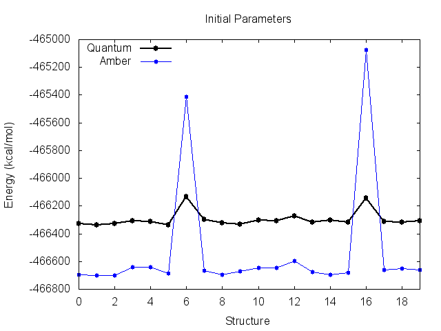
Before the fit, the Amber energies look like they match the quantum energies very well, but are shifted down the y-axis. This suggests an incorrect value of K. You can see why the derived K was incorrect however, as the energy of structures 6 and 16 are much higher than quantum.

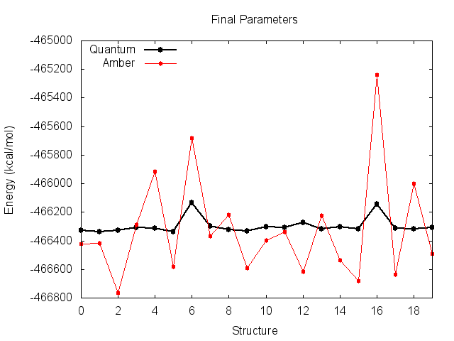
The final parameters attempt to compensate for the large energy difference for these two structures, resulting in small improvements, but messes up the entire trend for the remaining structures. It is clear that these two high-energy structures are significantly biasing the fit.

Visualize problem structures

We will use VMD to visualize the high energy structures. Open VMD, select New Molecule. Select a.prmtop as AMBER7 parm, then A_valid_structures.mdcrd as Amber Coordinates. This will load all of the structures.

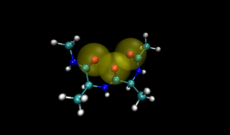
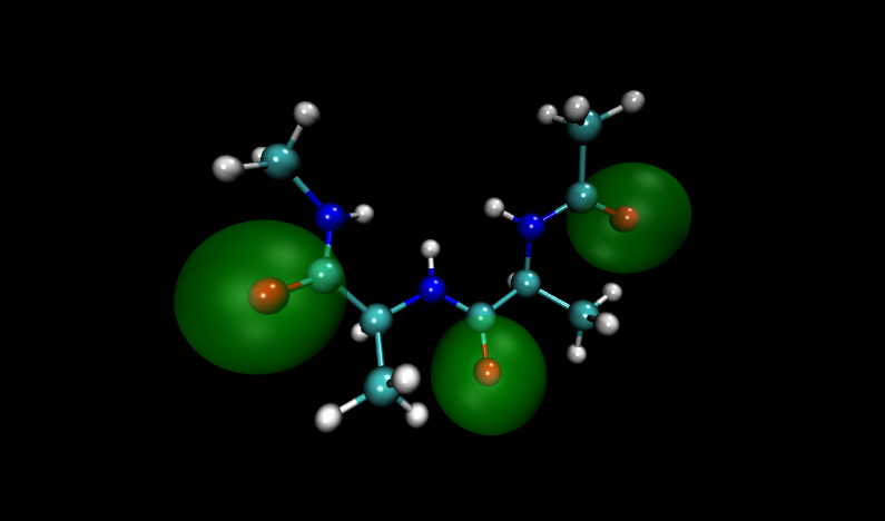
Navigate to the problem structures by entering 6 and 16 (VMD numbers from 0) into the frame box along the bottom of the molecule window. Compare these structures to others in the set. (Hint: add a representation of the VDW radii for oxygen atoms)

Visualizing these structures compared to others in the input file, it is clear that there is significant overlap between oxygen atoms in these two structures. Shown with VDW radii highlighted in yellow are the problem structures, compared to two others where it is shown in green.

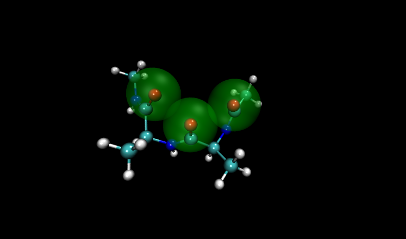
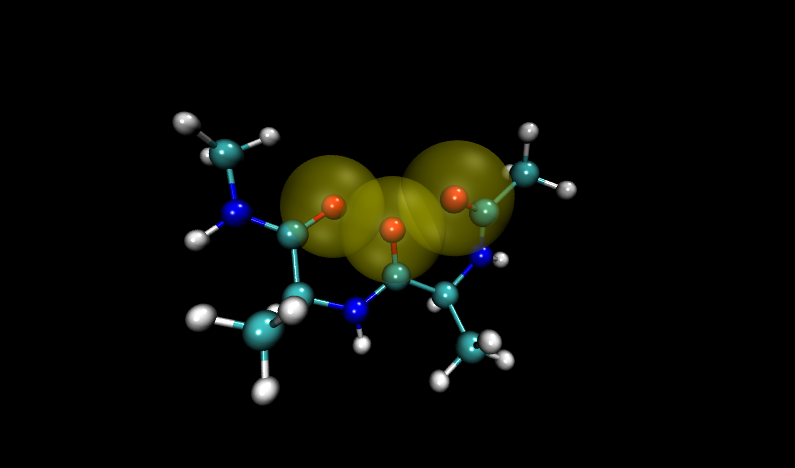Compare to two other structures, numbers 11 and 14:

Fortunately, Paramfit has functionality to handle this problem, which we will learn in the next section.